CostVolumeProfit Relationships Chapter 5 Power Point Authors Susan

Cost-Volume-Profit Relationships Chapter 5 Power. Point Authors: Susan Coomer Galbreath, Ph. D. , CPA Charles W. Caldwell, D. B. A. , CMA Jon A. Booker, Ph. D. , CPA, CIA Cynthia J. Rooney, Ph. D. , CPA Copyright © 2015 by Mc. Graw-Hill Education. All rights reserved.

5 -2 Key Assumptions of CVP Analysis 1. Selling price is constant. 2. Costs are linear and can be accurately divided into variable (constant per unit) and fixed (constant in total) elements. 3. In multiproduct companies, the sales mix is constant. 4. In manufacturing companies, inventories do not change (units produced = units sold).

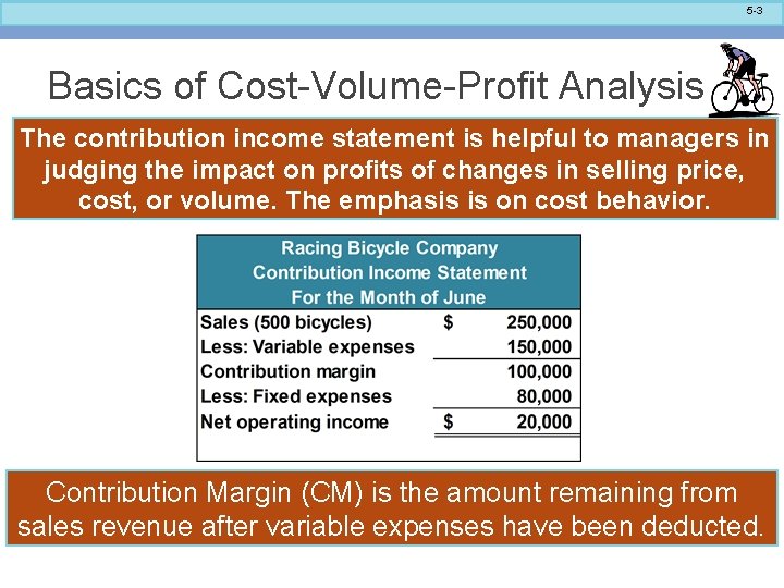
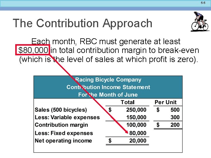
5 -3 Basics of Cost-Volume-Profit Analysis The contribution income statement is helpful to managers in judging the impact on profits of changes in selling price, cost, or volume. The emphasis is on cost behavior. Contribution Margin (CM) is the amount remaining from sales revenue after variable expenses have been deducted.

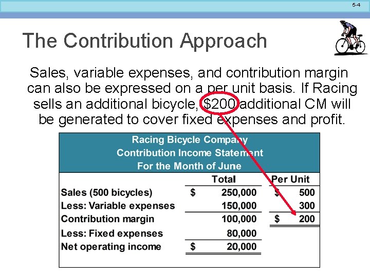
5 -4 The Contribution Approach Sales, variable expenses, and contribution margin can also be expressed on a per unit basis. If Racing sells an additional bicycle, $200 additional CM will be generated to cover fixed expenses and profit.

5 -5 The Contribution Approach Each month, RBC must generate at least $80, 000 in total contribution margin to break-even (which is the level of sales at which profit is zero).

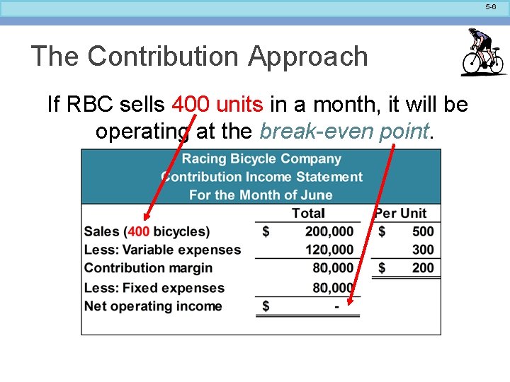
5 -6 The Contribution Approach If RBC sells 400 units in a month, it will be operating at the break-even point.

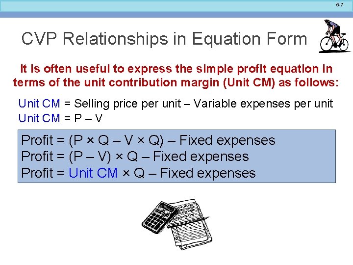
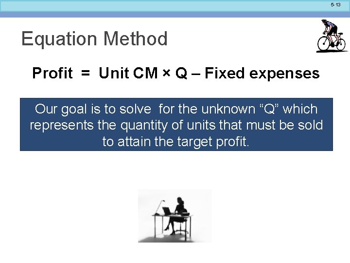
5 -7 CVP Relationships in Equation Form It is often useful to express the simple profit equation in terms of the unit contribution margin (Unit CM) as follows: Unit CM = Selling price per unit – Variable expenses per unit Unit CM = P – V Profit = (P × Q – V × Q) – Fixed expenses Profit = (P – V) × Q – Fixed expenses Profit = Unit CM × Q – Fixed expenses

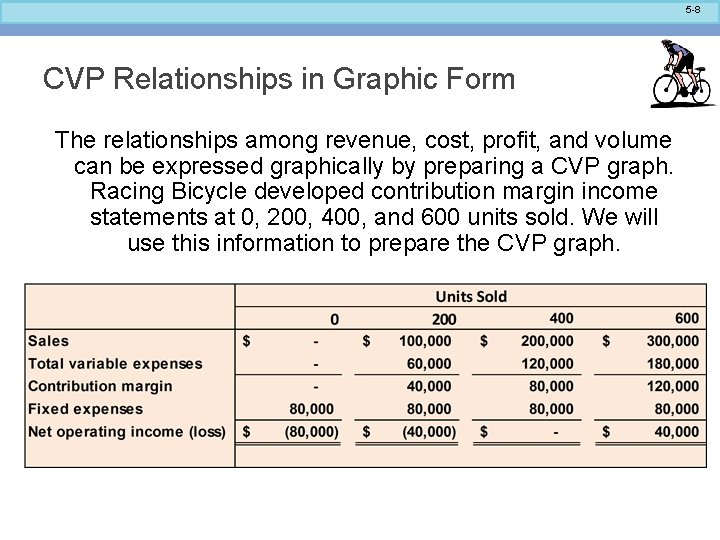
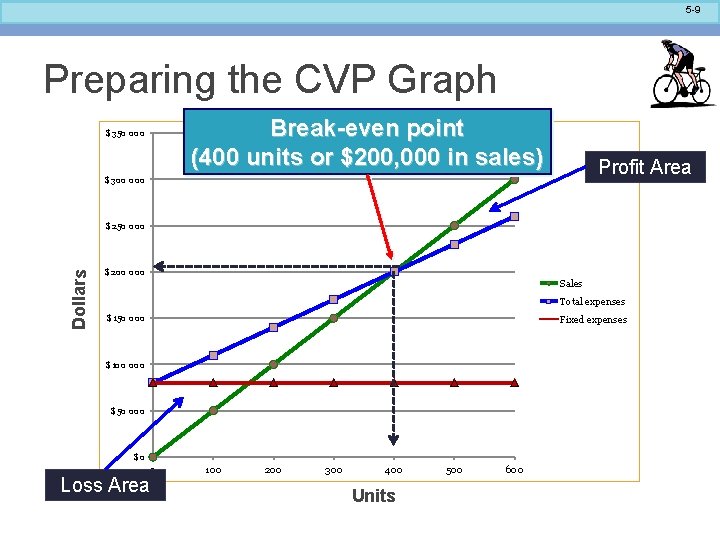
5 -8 CVP Relationships in Graphic Form The relationships among revenue, cost, profit, and volume can be expressed graphically by preparing a CVP graph. Racing Bicycle developed contribution margin income statements at 0, 200, 400, and 600 units sold. We will use this information to prepare the CVP graph.

5 -9 Preparing the CVP Graph Break-even point (400 units or $200, 000 in sales) $350 000 Profit Area $300 000 Dollars $250 000 $200 000 Sales Total expenses $150 000 Fixed expenses $100 000 $50 000 $0 0 Loss Area 100 200 300 400 Units 500 600

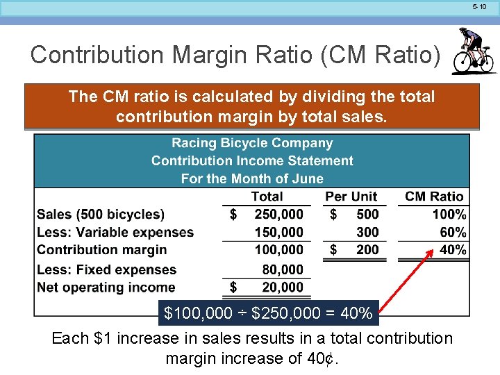
5 -10 Contribution Margin Ratio (CM Ratio) The CM ratio is calculated by dividing the total contribution margin by total sales. $100, 000 ÷ $250, 000 = 40% Each $1 increase in sales results in a total contribution margin increase of 40¢.

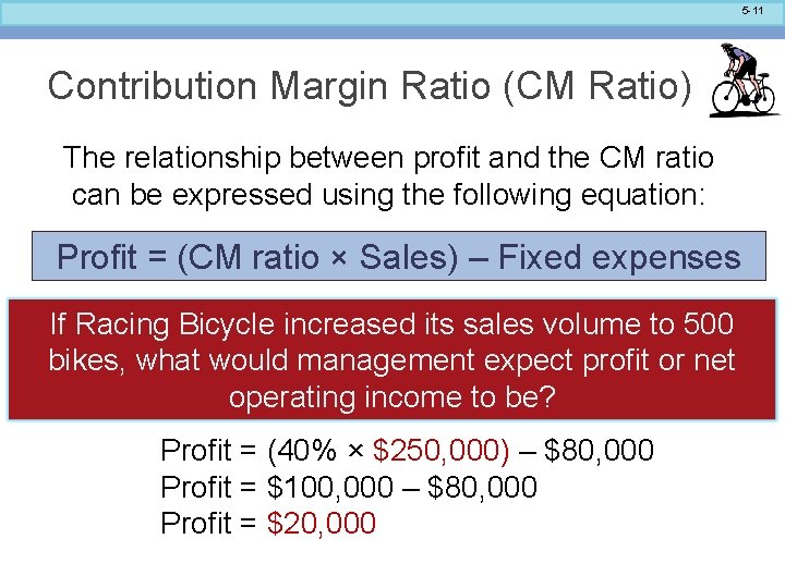
5 -11 Contribution Margin Ratio (CM Ratio) The relationship between profit and the CM ratio can be expressed using the following equation: Profit = (CM ratio × Sales) – Fixed expenses If Racing Bicycle increased its sales volume to 500 bikes, what would management expect profit or net operating income to be? Profit = (40% × $250, 000) – $80, 000 Profit = $100, 000 – $80, 000 Profit = $20, 000

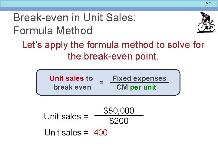
5 -12 Break-even in Unit Sales: Formula Method Let’s apply the formula method to solve for the break-even point. Unit sales to = break even Fixed expenses CM per unit $80, 000 Unit sales = $200 Unit sales = 400

5 -13 Equation Method Profit = Unit CM × Q – Fixed expenses Our goal is to solve for the unknown “Q” which represents the quantity of units that must be sold to attain the target profit.

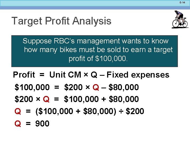
5 -14 Target Profit Analysis Suppose RBC’s management wants to know how many bikes must be sold to earn a target profit of $100, 000. Profit = Unit CM × Q – Fixed expenses $100, 000 = $200 × Q – $80, 000 $200 × Q = $100, 000 + $80, 000 Q = ($100, 000 + $80, 000) ÷ $200 Q = 900

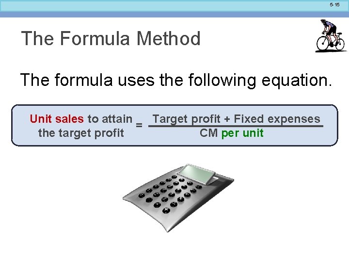
5 -15 The Formula Method The formula uses the following equation. Unit sales to attain Target profit + Fixed expenses = the target profit CM per unit

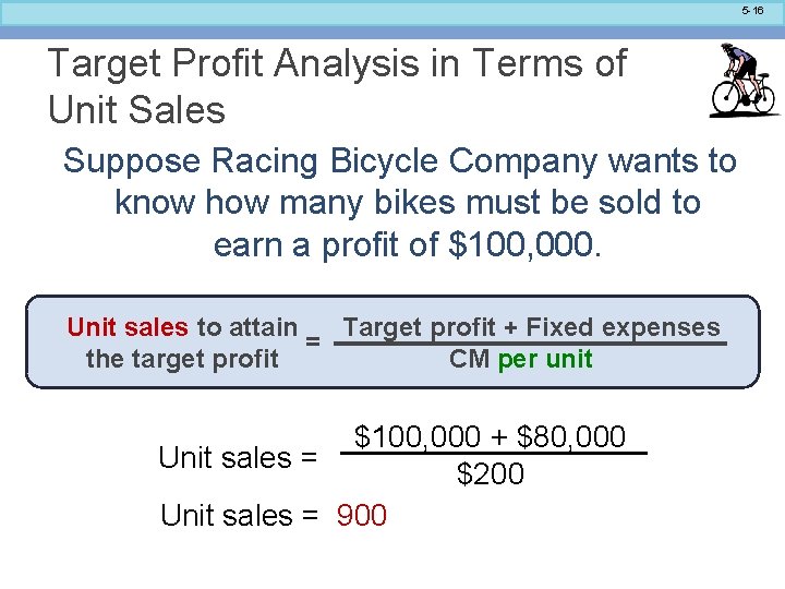
5 -16 Target Profit Analysis in Terms of Unit Sales Suppose Racing Bicycle Company wants to know how many bikes must be sold to earn a profit of $100, 000. Unit sales to attain Target profit + Fixed expenses = the target profit CM per unit $100, 000 + $80, 000 Unit sales = $200 Unit sales = 900

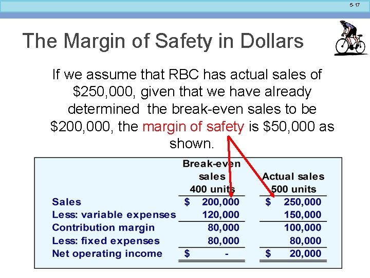
5 -17 The Margin of Safety in Dollars If we assume that RBC has actual sales of $250, 000, given that we have already determined the break-even sales to be $200, 000, the margin of safety is $50, 000 as shown.

5 -18 Cost Structure and Profit Stability Cost structure refers to the relative proportion of fixed and variable costs in an organization. Managers often have some latitude in determining their organization’s cost structure.

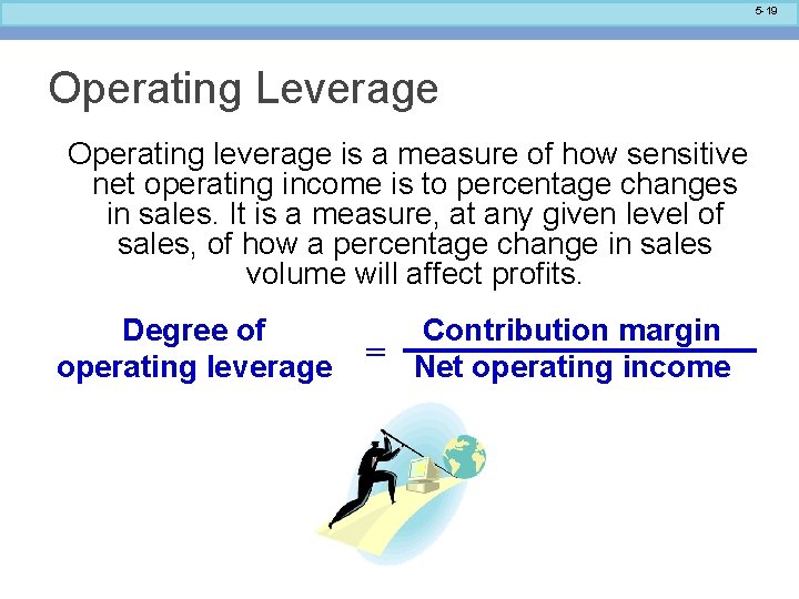
5 -19 Operating Leverage Operating leverage is a measure of how sensitive net operating income is to percentage changes in sales. It is a measure, at any given level of sales, of how a percentage change in sales volume will affect profits. Degree of operating leverage Contribution margin = Net operating income

5 -20 End of Chapter 5