Cost Sensitive Learning and Minimal Description Length Principle

Cost Sensitive Learning and Minimal Description Length Principle Lecture 18 Courtesy to Drs. . H. Witten, E. Frank and M. A. Hall

Counting the cost In practice, different types of classification errors often incur different costs ● Examples: ● ● Terrorist profiling “Not a terrorist” correct 99. 99% of the time Loan decisions Oil-slick detection Fault diagnosis Promotional mailing 2 Data Mining: Practical Machine Learning Tools and Techniques (Chapter 5)

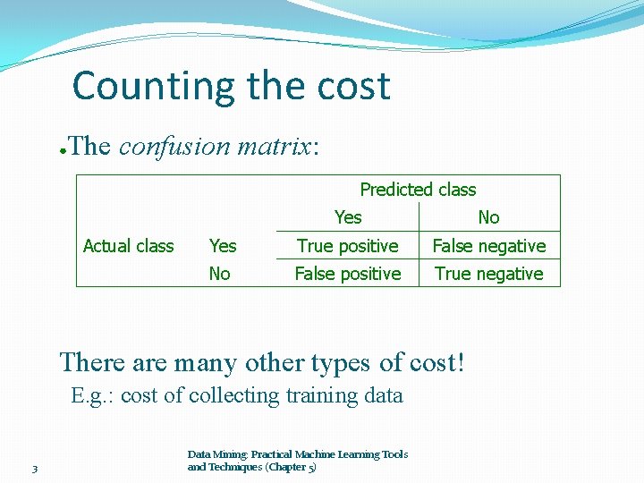
Counting the cost ● The confusion matrix: Predicted class Actual class Yes No Yes True positive False negative No False positive True negative There are many other types of cost! E. g. : cost of collecting training data 3 Data Mining: Practical Machine Learning Tools and Techniques (Chapter 5)

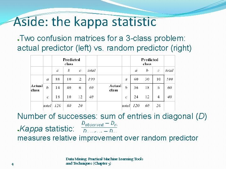
Aside: the kappa statistic Two confusion matrices for a 3 -class problem: actual predictor (left) vs. random predictor (right) ● Number of successes: sum of entries in diagonal (D) ● Kappa statistic: measures relative improvement over random predictor 4 Data Mining: Practical Machine Learning Tools and Techniques (Chapter 5)

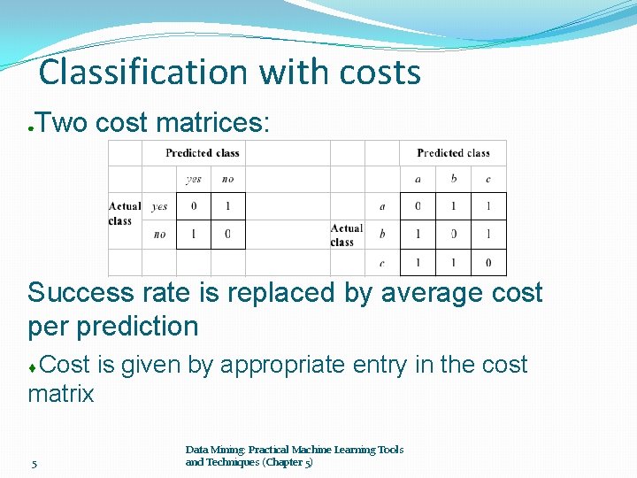
Classification with costs Two cost matrices: ● Success rate is replaced by average cost per prediction Cost is given by appropriate entry in the cost matrix 5 Data Mining: Practical Machine Learning Tools and Techniques (Chapter 5)

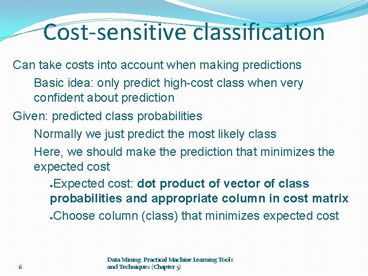
Cost-sensitive classification Can take costs into account when making predictions Basic idea: only predict high-cost class when very confident about prediction Given: predicted class probabilities Normally we just predict the most likely class Here, we should make the prediction that minimizes the expected cost ●Expected cost: dot product of vector of class probabilities and appropriate column in cost matrix ●Choose column (class) that minimizes expected cost 6 Data Mining: Practical Machine Learning Tools and Techniques (Chapter 5)

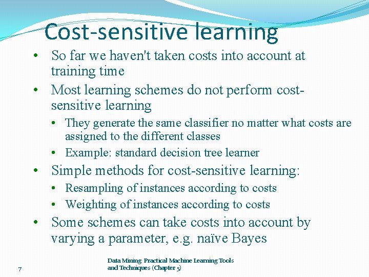
Cost-sensitive learning • So far we haven't taken costs into account at training time • Most learning schemes do not perform costsensitive learning • They generate the same classifier no matter what costs are assigned to the different classes • Example: standard decision tree learner • Simple methods for cost-sensitive learning: • Resampling of instances according to costs • Weighting of instances according to costs • Some schemes can take costs into account by varying a parameter, e. g. naïve Bayes 7 Data Mining: Practical Machine Learning Tools and Techniques (Chapter 5)

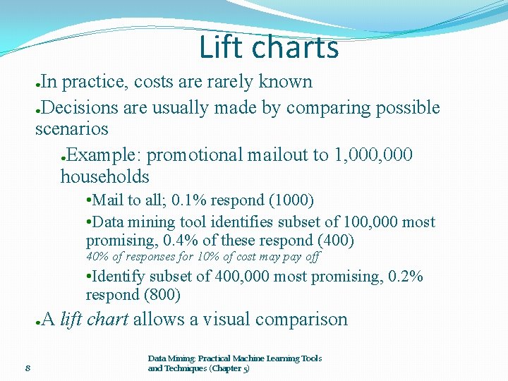
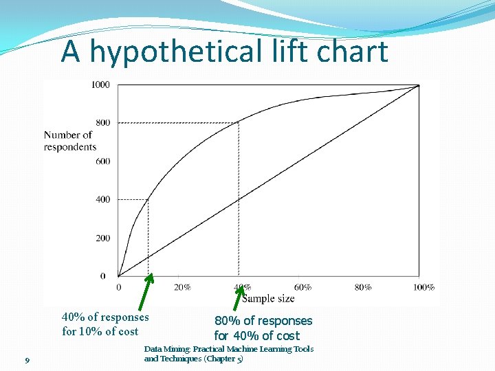
Lift charts In practice, costs are rarely known ●Decisions are usually made by comparing possible scenarios ●Example: promotional mailout to 1, 000 households ● • Mail to all; 0. 1% respond (1000) • Data mining tool identifies subset of 100, 000 most promising, 0. 4% of these respond (400) 40% of responses for 10% of cost may pay off • Identify subset of 400, 000 most promising, 0. 2% respond (800) A lift chart allows a visual comparison ● 8 Data Mining: Practical Machine Learning Tools and Techniques (Chapter 5)

A hypothetical lift chart 40% of responses for 10% of cost 9 80% of responses for 40% of cost Data Mining: Practical Machine Learning Tools and Techniques (Chapter 5)

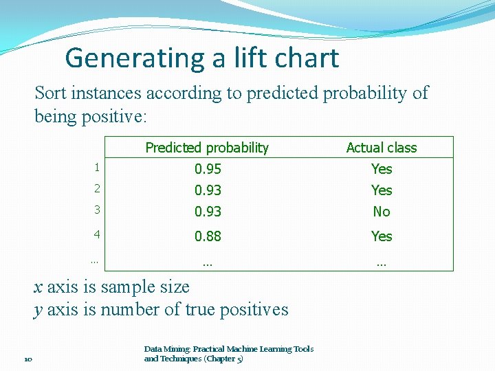
Generating a lift chart Sort instances according to predicted probability of being positive: Predicted probability Actual class 1 0. 95 Yes 2 0. 93 Yes 3 0. 93 No 4 0. 88 Yes … … … x axis is sample size y axis is number of true positives 10 Data Mining: Practical Machine Learning Tools and Techniques (Chapter 5)

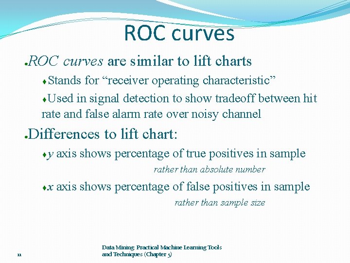
ROC curves are similar to lift charts ● Stands for “receiver operating characteristic” Used in signal detection to show tradeoff between hit rate and false alarm rate over noisy channel Differences to lift chart: ● y axis shows percentage of true positives in sample rather than absolute number x axis shows percentage of false positives in sample rather than sample size 11 Data Mining: Practical Machine Learning Tools and Techniques (Chapter 5)

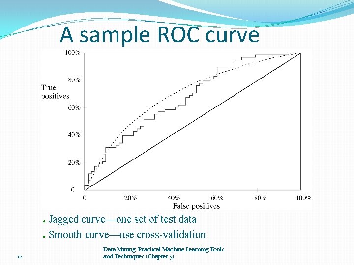
A sample ROC curve Jagged curve—one set of test data ● Smooth curve—use cross-validation ● 12 Data Mining: Practical Machine Learning Tools and Techniques (Chapter 5)

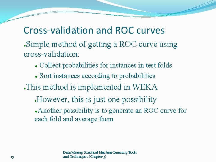
Cross-validation and ROC curves Simple method of getting a ROC curve using cross-validation: ● Collect probabilities for instances in test folds Sort instances according to probabilities ● This method is implemented in WEKA ●However, this is just one possibility Another possibility is to generate an ROC curve for each fold and average them 13 Data Mining: Practical Machine Learning Tools and Techniques (Chapter 5)

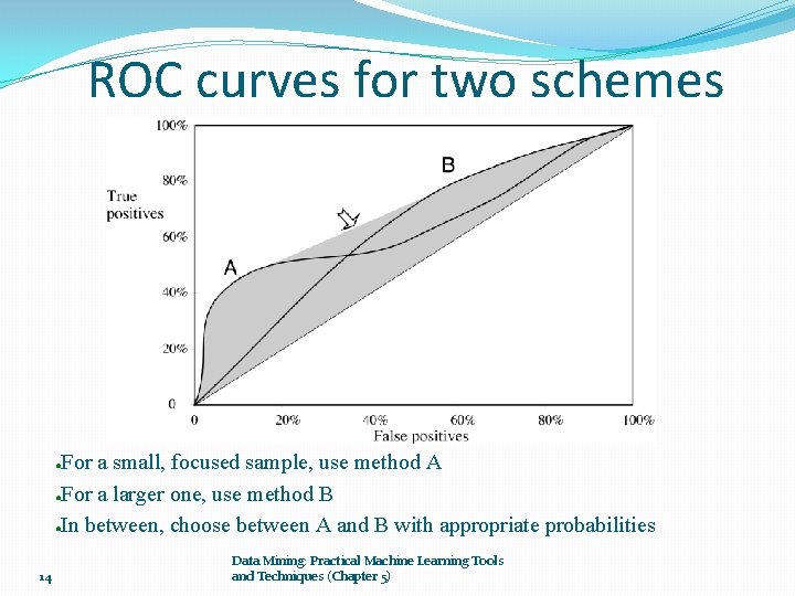
ROC curves for two schemes For a small, focused sample, use method A ●For a larger one, use method B ●In between, choose between A and B with appropriate probabilities ● 14 Data Mining: Practical Machine Learning Tools and Techniques (Chapter 5)

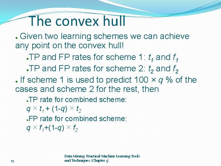
The convex hull Given two learning schemes we can achieve any point on the convex hull! ●TP and FP rates for scheme 1: t and f 1 1 ●TP and FP rates for scheme 2: t and f 2 2 ● If scheme 1 is used to predict 100 × q % of the cases and scheme 2 for the rest, then ● TP rate for combined scheme: q × t 1 + (1 -q) × t 2 ●FP rate for combined scheme: q × f 1+(1 -q) × f 2 ● 15 Data Mining: Practical Machine Learning Tools and Techniques (Chapter 5)

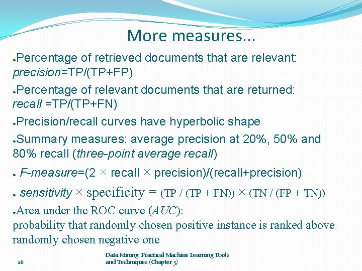
More measures. . . Percentage of retrieved documents that are relevant: precision=TP/(TP+FP) ●Percentage of relevant documents that are returned: recall =TP/(TP+FN) ●Precision/recall curves have hyperbolic shape ●Summary measures: average precision at 20%, 50% and 80% recall (three-point average recall) ● ● F-measure=(2 × recall × precision)/(recall+precision) sensitivity × specificity = (TP / (TP + FN)) × (TN / (FP + TN)) ●Area under the ROC curve (AUC): probability that randomly chosen positive instance is ranked above randomly chosen negative one ● 16 Data Mining: Practical Machine Learning Tools and Techniques (Chapter 5)

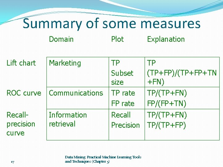
Summary of some measures Domain Plot Explanation Lift chart Marketing TP (TP+FP)/(TP+FP+TN +FN) ROC curve Communications TP Subset size TP rate FP rate Recallprecision curve Information retrieval 17 TP/(TP+FN) FP/(FP+TN) Recall TP/(TP+FN) Precision TP/(TP+FP) Data Mining: Practical Machine Learning Tools and Techniques (Chapter 5)

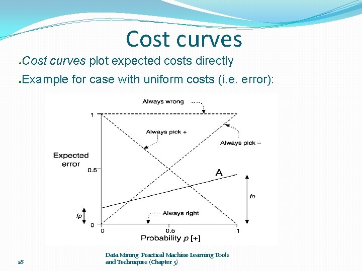
Cost curves ● Cost curves plot expected costs directly ● Example for case with uniform costs (i. e. error): 18 Data Mining: Practical Machine Learning Tools and Techniques (Chapter 5)

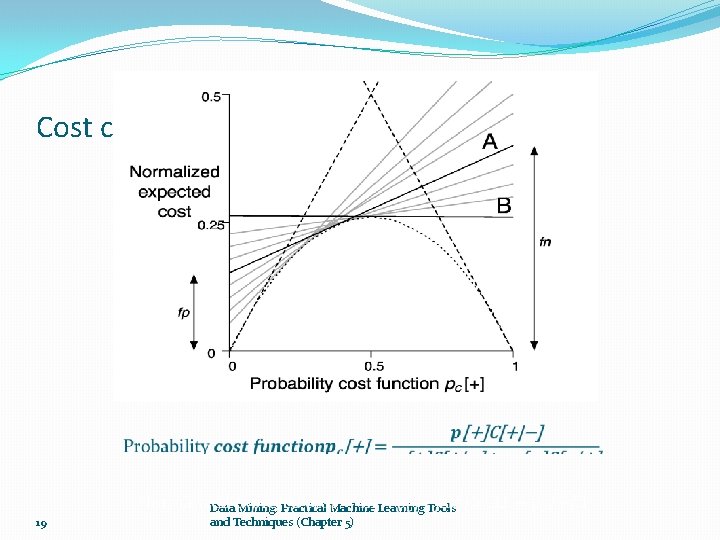
Cost curves: example with costs 19 Data Mining: Practical Machine Learning Tools and Techniques (Chapter 5)

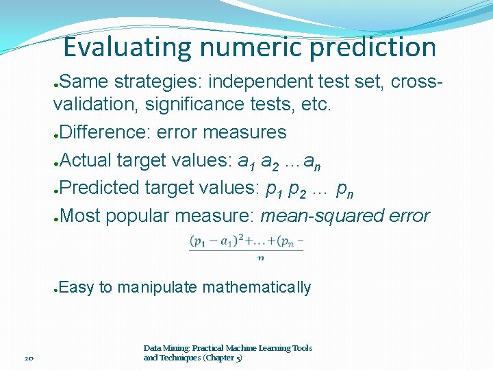
Evaluating numeric prediction Same strategies: independent test set, crossvalidation, significance tests, etc. ●Difference: error measures ●Actual target values: a a …a 1 2 n ●Predicted target values: p p … p 1 2 n ●Most popular measure: mean-squared error ● ● 20 Easy to manipulate mathematically Data Mining: Practical Machine Learning Tools and Techniques (Chapter 5)

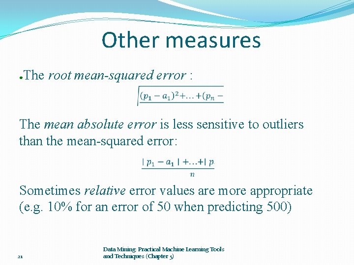
Other measures The root mean-squared error : ● The mean absolute error is less sensitive to outliers than the mean-squared error: Sometimes relative error values are more appropriate (e. g. 10% for an error of 50 when predicting 500) 21 Data Mining: Practical Machine Learning Tools and Techniques (Chapter 5)

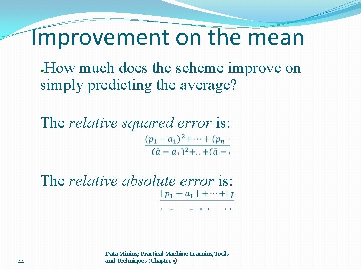
Improvement on the mean How much does the scheme improve on simply predicting the average? ● The relative squared error is: The relative absolute error is: 22 Data Mining: Practical Machine Learning Tools and Techniques (Chapter 5)

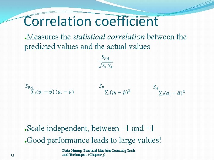
Correlation coefficient Measures the statistical correlation between the predicted values and the actual values ● Scale independent, between – 1 and +1 ●Good performance leads to large values! ● 23 Data Mining: Practical Machine Learning Tools and Techniques (Chapter 5)

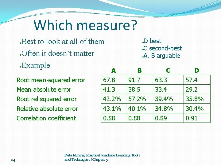
Which measure? 24 ● Best to look at all of them ● Often it doesn’t matter ● Example: D best ●C second-best ●A, B arguable ● A B Root mean-squared error 67. 8 91. 7 63. 3 57. 4 Mean absolute error 41. 3 38. 5 33. 4 29. 2 Root rel squared error 42. 2% 57. 2% 39. 4% 35. 8% Relative absolute error 43. 1% 40. 1% 34. 8% 30. 4% Correlation coefficient 0. 88 0. 89 0. 91 Data Mining: Practical Machine Learning Tools and Techniques (Chapter 5) C D

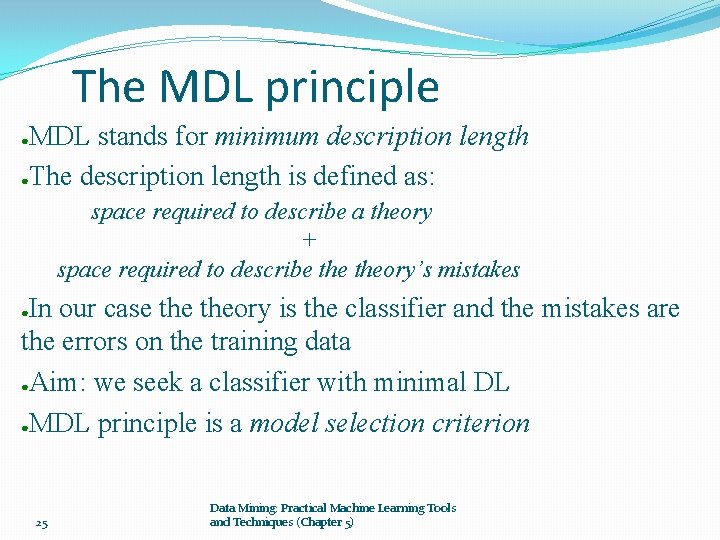
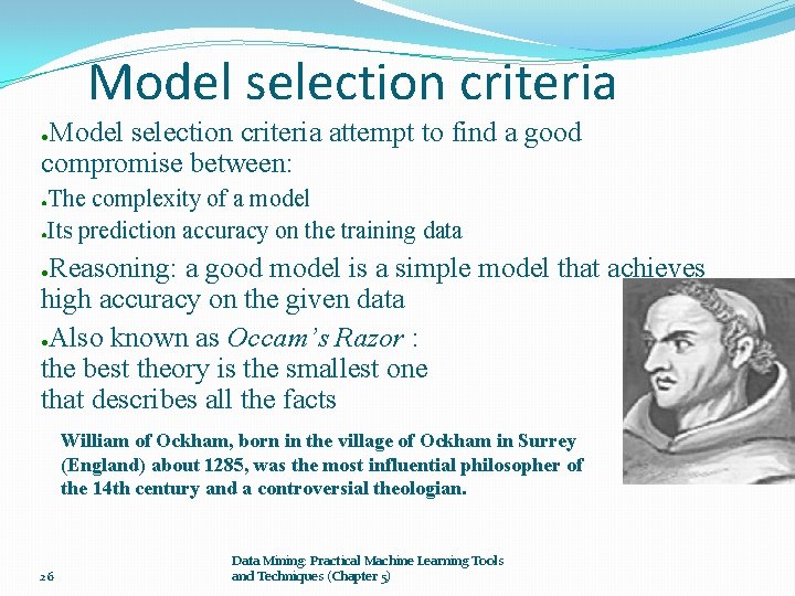
The MDL principle MDL stands for minimum description length ●The description length is defined as: ● space required to describe a theory + space required to describe theory’s mistakes In our case theory is the classifier and the mistakes are the errors on the training data ●Aim: we seek a classifier with minimal DL ●MDL principle is a model selection criterion ● 25 Data Mining: Practical Machine Learning Tools and Techniques (Chapter 5)

Model selection criteria attempt to find a good compromise between: ● The complexity of a model ●Its prediction accuracy on the training data ● Reasoning: a good model is a simple model that achieves high accuracy on the given data ●Also known as Occam’s Razor : the best theory is the smallest one that describes all the facts ● William of Ockham, born in the village of Ockham in Surrey (England) about 1285, was the most influential philosopher of the 14 th century and a controversial theologian. 26 Data Mining: Practical Machine Learning Tools and Techniques (Chapter 5)

Elegance vs. errors Theory 1: very simple, elegant theory that explains the data almost perfectly ●Theory 2: significantly more complex theory that reproduces the data without mistakes ●Theory 1 is probably preferable ●Classical example: Kepler’s three laws on planetary motion ● Less accurate than Copernicus’s latest refinement of the Ptolemaic theory of epicycles 27 Data Mining: Practical Machine Learning Tools and Techniques (Chapter 5)

MDL and compression MDL principle relates to data compression: ● The best theory is the one that compresses the data the most ●I. e. to compress a dataset we generate a model and then store the model and its mistakes ● We need to compute (a) size of the model, and (b) space needed to encode the errors ●(b) easy: use the informational loss function ●(a) need a method to encode the model ● 28 Data Mining: Practical Machine Learning Tools and Techniques (Chapter 5)

MDL and Bayes’s theorem L[T]=“length” of theory ●L[E|T]=training set encoded wrt theory ●Description length= L[T] + L[E|T] ●Bayes’s theorem gives a posteriori probability of a theory given the data: ● Equivalent to: 29 Data Mining: Practical Machine Learning Tools and Techniques (Chapter 5) constant

MDL and MAP stands for maximum a posteriori probability ●Finding the MAP theory corresponds to finding the MDL theory ●Difficult bit in applying the MAP principle: determining the prior probability Pr[T] of theory ●Corresponds to difficult part in applying the MDL principle: coding scheme for theory ●I. e. if we know a priori that a particular theory is more likely we need fewer bits to encode it ● 30 Data Mining: Practical Machine Learning Tools and Techniques (Chapter 5)

Discussion of MDL principle Advantage: makes full use of the training data when selecting a model ●Disadvantage 1: appropriate coding scheme/prior probabilities for theories are crucial ●Disadvantage 2: no guarantee that the MDL theory is the one which minimizes the expected error ●Note: Occam’s Razor is an axiom! ●Epicurus’s principle of multiple explanations: keep all theories that are consistent with the data ● 31 Data Mining: Practical Machine Learning Tools and Techniques (Chapter 5)

MDL and clustering Description length of theory: bits needed to encode the clusters ● e. g. cluster centers Description length of data given theory: encode cluster membership and position relative to cluster ● e. g. distance to cluster center Works if coding scheme uses less code space for small numbers than for large ones ●With nominal attributes, must communicate probability distributions for each cluster ● 32 Data Mining: Practical Machine Learning Tools and Techniques (Chapter 5)