Cost Estimating Basics Adapted from CEBo K Modules

Cost Estimating Basics Adapted from CEBo. K Modules 1 and 2 Kevin Cincotta, CCEA, PMP Cassandra M. Capots, PCEA Prepared for: 2016 ICEAA Canada Workshop February 22 -23, 2016 Ottawa, ON

v 1. 2 Acknowledgments • ICEAA is indebted to TASC, Inc. , for the development and maintenance of the Cost Estimating Body of Knowledge (CEBo. K®) – ICEAA is also indebted to Technomics, Inc. , for the independent review and maintenance of CEBo. K® • ICEAA is also indebted to the following individuals who have made significant contributions to the development, review, and maintenance of Cost. PROF and CEBo. K ® • Module 2 Cost Estimating Techniques – Lead authors: Crystal H. Rudloff, Kenneth D. Odom, Colleen M. Craig – Assistant author: Daniel V. Cota – Senior reviewers: Richard L. Coleman, Richard B. Collins II, Fred K. Blackburn, Kevin Cincotta – Reviewer: Laurette Sullivan, Karyn L. Sanders – Managing editor: Peter J. Braxton Unit I - Module 2 © 2002 -2013 ICEAA. All rights reserved. 2

v 1. 2 Cost Estimating • Cost Estimating: – The process of collecting and analyzing historical data and applying quantitative models, techniques, tools, and databases to predict the future cost of an item, product, program, or task • Purpose of cost estimating – Translate system/functional requirements associated with programs, projects, proposals, or processes into budget requirements – Determine and communicate a realistic view of the likely cost outcome, which can form the basis of the plan for executing the work “Suppose one of you wants to build a tower. Will he not first sit down and estimate the cost to see if he has enough money to complete it? For if he lays the foundation and is not able to finish it, everyone who sees it will ridicule him, saying, ‘This fellow began to build and was not able to finish. ’” -Jesus Christ, Luke 14: 28 -30 Unit I - Module 1 © 2002 -2013 ICEAA. All rights reserved. 3

Motivations for Cost Estimating • Budgeting – (Independent) Cost Estimates to establish program budgets should give a reasonable chance of “success” • Measured by Track Record 14 15 • Planning – Bases of Estimate (BOEs) to establish project baselines should allow an accurate measurement of progress • Measured by EVM Performance Indices • Trade-Offs 13 16 – Parametric Models and Cost Response Curves (CRCs) to give quick and accurate estimates should guide system requirements and design toward affordability • Measured by periodic Life Cycle Cost Estimates (LCCEs) Tip: Proper treatment of Risk is crucial to all three! Unit I - Module 1 © 2002 -2013 ICEAA. All rights reserved. 9 4 v 1. 2

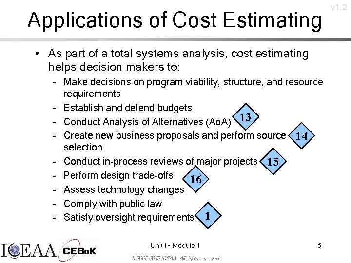
Applications of Cost Estimating • As part of a total systems analysis, cost estimating helps decision makers to: – Make decisions on program viability, structure, and resource requirements – Establish and defend budgets – Conduct Analysis of Alternatives (Ao. A) 13 – Create new business proposals and perform source 14 selection – Conduct in-process reviews of major projects 15 – Perform design trade-offs 16 – Assess technology changes – Comply with public law – Satisfy oversight requirements 1 Unit I - Module 1 © 2002 -2013 ICEAA. All rights reserved. 5 v 1. 2

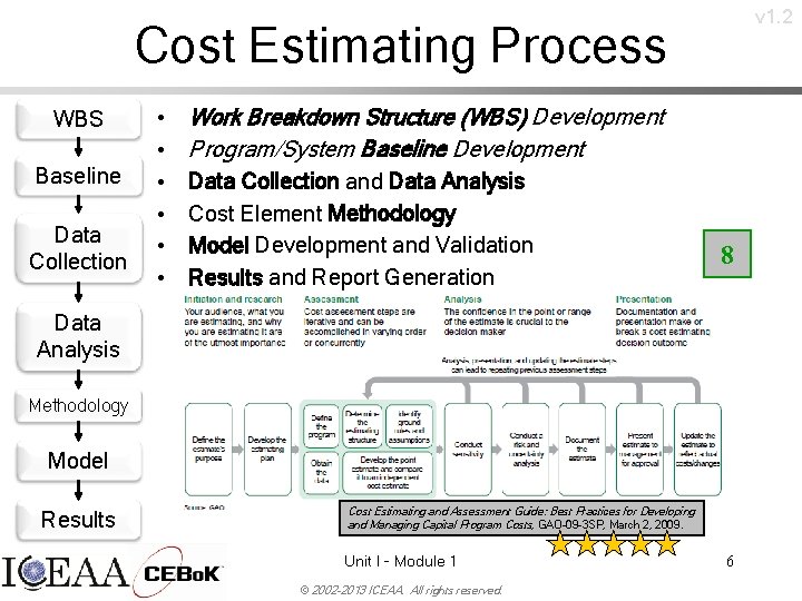
v 1. 2 Cost Estimating Process WBS Baseline Data Collection • • • Work Breakdown Structure (WBS) Development Program/System Baseline Development Data Collection and Data Analysis Cost Element Methodology Model Development and Validation Results and Report Generation 8 Data Analysis Methodology Model Results Cost Estimating and Assessment Guide: Best Practices for Developing and Managing Capital Program Costs, GAO-09 -3 SP, March 2, 2009. Unit I - Module 1 © 2002 -2013 ICEAA. All rights reserved. 6

v 1. 2 Unit Index Unit I – Cost Estimating 1. Cost Estimating Basics 2. Cost Estimating Techniques 3. Parametric Estimating Unit II – Cost Analysis Techniques Unit III – Analytical Methods Unit IV – Specialized Costing Unit V – Management Applications Unit I - Module 2 © 2002 -2013 ICEAA. All rights reserved. 7

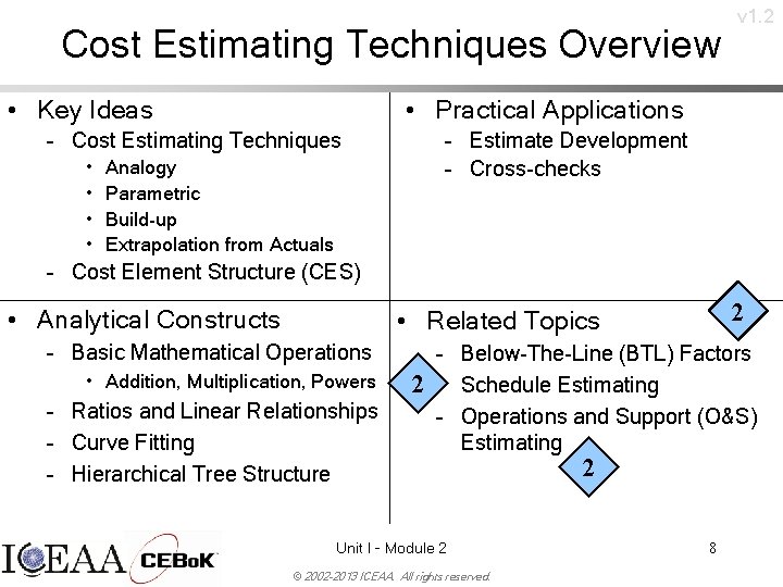
Cost Estimating Techniques Overview • Key Ideas • Practical Applications – Cost Estimating Techniques • • v 1. 2 Analogy Parametric Build-up Extrapolation from Actuals – Estimate Development – Cross-checks – Cost Element Structure (CES) • Analytical Constructs 2 • Related Topics – Basic Mathematical Operations • Addition, Multiplication, Powers – Ratios and Linear Relationships – Curve Fitting – Hierarchical Tree Structure – Below-The-Line (BTL) Factors 2 – Schedule Estimating – Operations and Support (O&S) Estimating Unit I - Module 2 © 2002 -2013 ICEAA. All rights reserved. 2 8

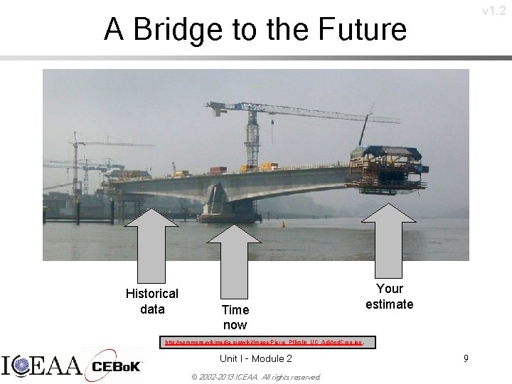
v 1. 2 A Bridge to the Future Historical data Time now Your estimate http: //commons. wikimedia. org/wiki/Image: Pierre_Pflimlin_UC_Adj. And. Crop. jpg. Unit I - Module 2 © 2002 -2013 ICEAA. All rights reserved. 9

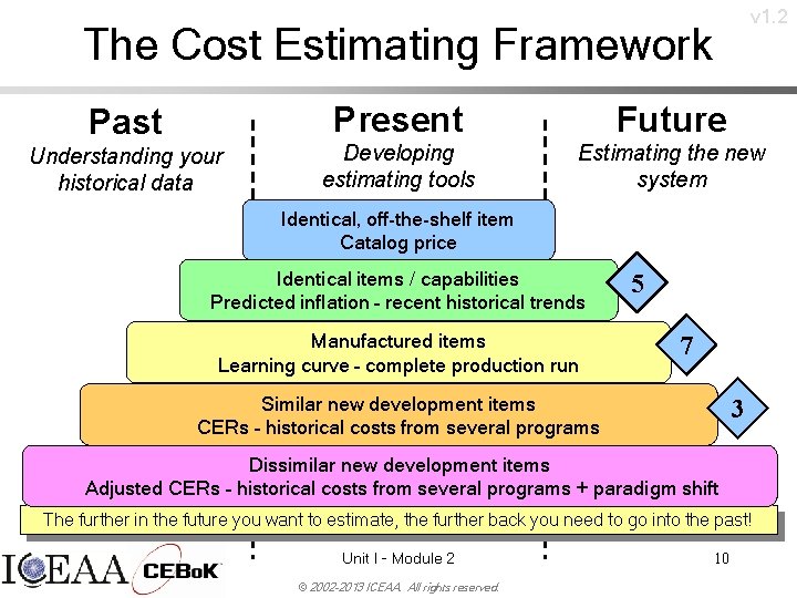
v 1. 2 The Cost Estimating Framework Past Understanding your historical data Present Future Developing estimating tools Estimating the new system Identical, off-the-shelf item Catalog price Identical items / capabilities Predicted inflation – recent historical trends Manufactured items Learning curve – complete production run 5 7 Similar new development items CERs – historical costs from several programs 3 Dissimilar new development items Adjusted CERs – historical costs from several programs + paradigm shift The further in the future you want to estimate, the further back you need to go into the past! Unit I - Module 2 © 2002 -2013 ICEAA. All rights reserved. 10

Cost Estimating Techniques Outline • Core Knowledge – – – Introduction Uncertainty and Risk Cost Estimating Techniques Using Cost Estimating Techniques Comparison of Techniques • Summary • Resources • Related and Advanced Topics Unit I - Module 2 © 2002 -2013 ICEAA. All rights reserved. 11 v 1. 2

v 1. 2 Introduction • The four essential cost estimating techniques (or methodologies) are: 11 – – Analogy Parametric Build-Up Extrapolation from Actuals • Other topics will be discussed in relation to the four essential techniques – Expert Opinion Unit I - Module 2 © 2002 -2013 ICEAA. All rights reserved. 12

v 1. 2 Risk Terminology 9 • Precision vs. accuracy – Precision = narrow range – Accuracy = range centered on “right” Tip: We want estimates to be both answer • Uncertainty vs. risk precise and accurate, but imprecisely accurate is better than precisely inaccurate! – Uncertainty = range of possible outcomes • Characterization of precision Correction of bias – Risk = shift of range to account for lack of accuracy of unadjusted estimates Warning: Uncertainty and risk are difficult but essential. Unit I - Module 2 © 2002 -2013 ICEAA. All rights reserved. 13

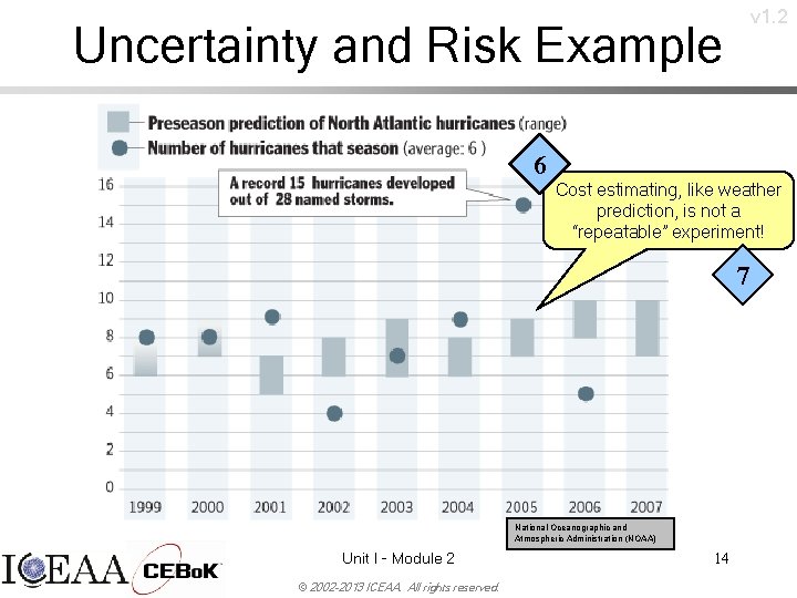
v 1. 2 Uncertainty and Risk Example 6 Cost estimating, like weather prediction, is not a “repeatable” experiment! 7 National Oceanographic and Atmospheric Administration (NOAA) Unit I - Module 2 © 2002 -2013 ICEAA. All rights reserved. 14

Uncertainty and Risk Illustration Estimate Based on an Average Tip: Estimating cost as an average of historical data is generally a good starting point Unit I - Module 2 © 2002 -2013 ICEAA. All rights reserved. 15 v 1. 2

v 1. 2 Cost Estimating Techniques • • Analogy Parametric Build-Up Extrapolation from Actuals

Cost Estimating Techniques Basics • Cost Estimating Techniques provide the structure of your cost estimate – They’re what enable you to predict future costs based on historical data – Techniques rely on statistical properties, logical relationships, and emotional appeal • Four essential types – – Analogy: “It’s like one of these” Parametric: “This pattern holds” Build-Up: “It’s made up of these” Extrapolation from Actuals: “Stay the course” Unit I - Module 2 © 2002 -2013 ICEAA. All rights reserved. 17 v 1. 2

v 1. 2 Analogy - Method • Comparative analysis of similar systems • Adjust costs of an analogous system to 3 estimate the new system, using a numeric ratio based on an intuitive physical or countable metric “It’s like one – e. g. , weight, SLOC, number of users of these” • Other adjustments may need to be made for any estimating methodology 5 – – Programmatic information (quantity/schedule) Government vs. Commercial practices AKA Comparison Contract specifics Technique, Ratio, $ Economic trends Analysis of Analogues Unit I - Module 2 © 2002 -2013 ICEAA. All rights reserved. $ 18

v 1. 2 Analogy - Application • Used early in the program life cycle – Data are not available to support using more detailed methods – Not enough data exist for a number of similar systems, but can find cost data from a single similar system • The best results are achieved when – Adjustments can be quantified – Subjective adjustments are minimized – Similarities between old and new systems are high 1. Minimize differences to one or more that can be scaled, then 2. Minimize the amount of scaling (size of adjustment factor) • Can be used as a cross check for other methods Unit I - Module 2 © 2002 -2013 ICEAA. All rights reserved. 19

v 1. 2 Analogy – Considerations • Strengths – Can be used early in programs before detailed requirements are known – Difficult to refute if there is strong resemblance • Weaknesses – No objective test of validity – Danger in choice of scaling factor • Which variable • Functional form (linear vs. non-linear scaling) • What slope (through origin or borrowed slope) • Challenges – Difficult to obtain cost/technical data on old/new systems for comparison Warning 1: An adjusted analogy is like a regression, but the slope is just a guess. Warning 2: An adjusted analogy is, by definition, estimating outside the range of the data. Unit I - Module 2 © 2002 -2013 ICEAA. All rights reserved. 20

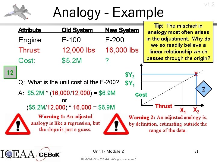
v 1. 2 Analogy - Example 12 Attribute Old System New System Engine: Thrust: Cost: F-100 12, 000 lbs $5. 2 M F-200 16, 000 lbs ? Tip: The mischief in analogy most often arises in the adjustment. Why do we so readily believe a linear relationship which passes through the origin? X $Y 2 Q: What is the unit cost of the F-200? $Y 1 A: $5. 2 M * (16, 000/12, 000) = $6. 9 M or ($5. 2 M/12, 000) * 16, 000 = $6. 9 M Warning 1: An adjusted analogy is like a regression, but the slope is just a guess. 2 Cost Thrust X 1 X 2 Warning 2: An adjusted analogy is, by definition, estimating outside the range of the data. Unit I - Module 2 © 2002 -2013 ICEAA. All rights reserved. 21

Analogy – Uncertainty and Risk • Uncertainty 9 – Uncertainty in point of departure – Uncertainty in slope of adjustment • Risk – Risks not “included” in analogy system – Historical growth of scaling quantity “Analogies: Techniques for Adjusting Them, ” R. L. Coleman, J. R. Summerville, S. S. Gupta, SCEA 2004. Unit I - Module 2 © 2002 -2013 ICEAA. All rights reserved. 22 v 1. 2

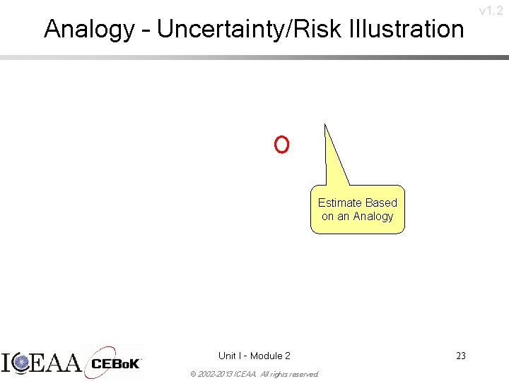
Analogy – Uncertainty/Risk Illustration Estimate Based on an Analogy Unit I - Module 2

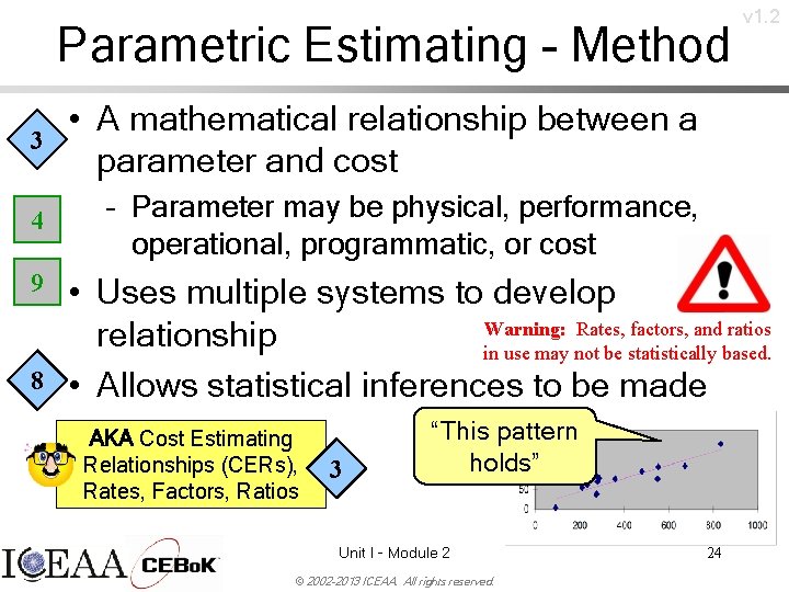
Parametric Estimating - Method 3 • A mathematical relationship between a parameter and cost 4 – Parameter may be physical, performance, operational, programmatic, or cost 9 8 v 1. 2 • Uses multiple systems to develop Warning: Rates, factors, and ratios relationship in use may not be statistically based. • Allows statistical inferences to be made AKA Cost Estimating Relationships (CERs), Rates, Factors, Ratios 3 “This pattern holds” Unit I - Module 2 © 2002 -2013 ICEAA. All rights reserved. 24

v 1. 2 Parametric Estimating - Application • Use of Parametrics 4 – Requires a good database which is relevant to the system being estimated – Excellent for use early in program life cycle before a detailed design exists – Used as the design progresses to capture changes • CAIV trades 16 • Good as a cross-check for other methods • • Unit I - Module 2 © 2002 -2013 ICEAA. All rights reserved. 25

Parametric Estimating – Considerations v 1. 2 • Strengths – Can be easily adjusted for changes by modifying input parameters – Sensitivity Analysis - Can show changes to certain parameters impact the cost 8 – Objective measures of validity – Statistical measures for uncertainty 9 • Weaknesses – “Black box syndrome” with pre-existing CERs, commercial models • Challenges 4 – Difficult to ensure consistency and validity of data • Goal is to establish and maintain homogeneous data set – Must constantly review relationships to ensure that relationships reflect current status of relevant programs, technology, and other 7 factors Unit I - Module 2 © 2002 -2013 ICEAA. All rights reserved. 26

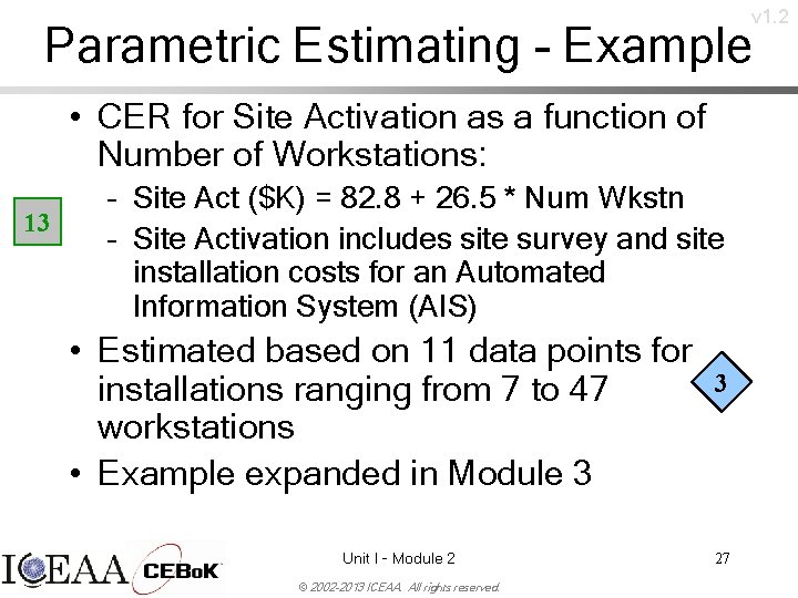
v 1. 2 Parametric Estimating - Example • CER for Site Activation as a function of Number of Workstations: 13 – Site Act ($K) = 82. 8 + 26. 5 * Num Wkstn – Site Activation includes site survey and site installation costs for an Automated Information System (AIS) • Estimated based on 11 data points for installations ranging from 7 to 47 workstations • Example expanded in Module 3 Unit I - Module 2 © 2002 -2013 ICEAA. All rights reserved. 3 27

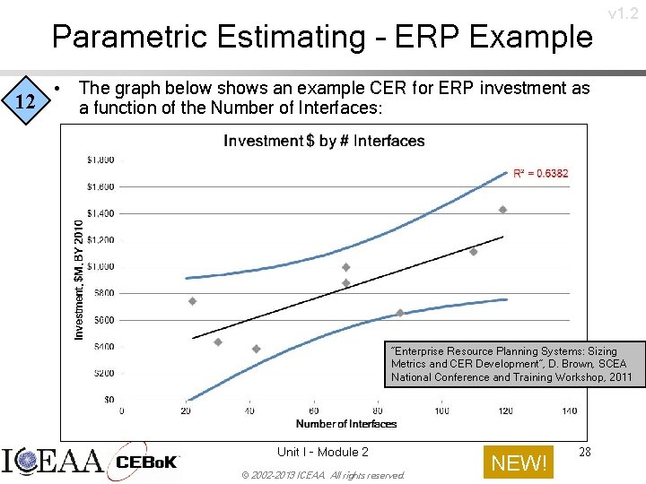
Parametric Estimating – ERP Example v 1. 2 • The graph below shows an example CER for ERP investment as 12 a function of the Number of Interfaces: “Enterprise Resource Planning Systems: Sizing Metrics and CER Development”, D. Brown, SCEA National Conference and Training Workshop, 2011 Unit I - Module 2 © 2002 -2013 ICEAA. All rights reserved. NEW! 28

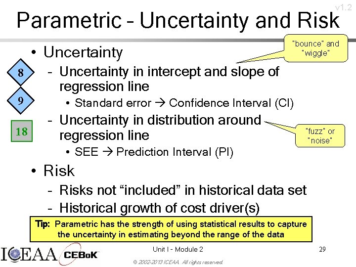
v 1. 2 Parametric – Uncertainty and Risk “bounce” and “wiggle” • Uncertainty 8 9 18 – Uncertainty in intercept and slope of regression line • Standard error Confidence Interval (CI) – Uncertainty in distribution around regression line • SEE Prediction Interval (PI) “fuzz” or “noise” • Risk – Risks not “included” in historical data set – Historical growth of cost driver(s) Tip: Parametric has the strength of using statistical results to capture the uncertainty in estimating beyond the range of the data Unit I - Module 2 © 2002 -2013 ICEAA. All rights reserved. 29

v 1. 2 Parametric – Uncertainty/Risk Illustration Estimate Based on a CER (Parametric) Unit

v 1. 2 Parametric – Uncertainty/Risk Illustration Calibrated CER Estimate Based on a Calibrated

Uncertainty and Risk Illustration Unit I - Module 2 © 2002 -2013 ICEAA. All

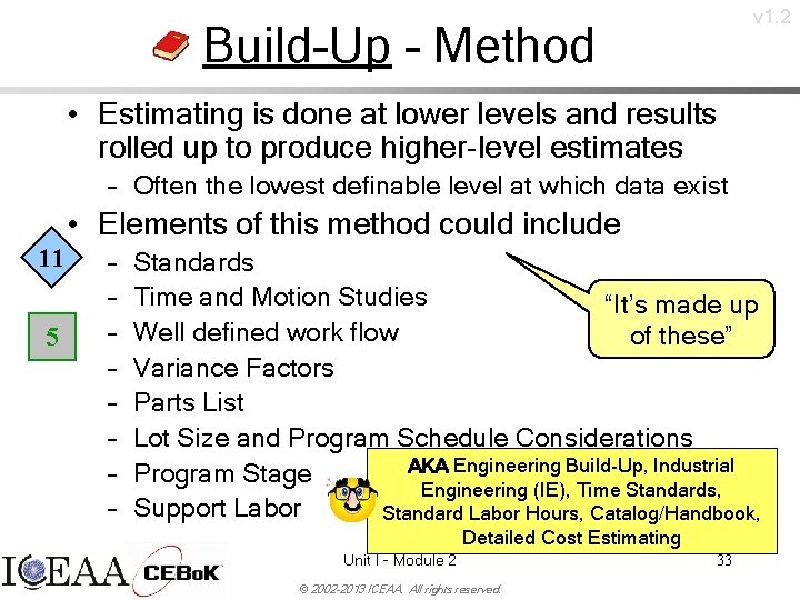
v 1. 2 Build-Up - Method • Estimating is done at lower levels and results rolled up to produce higher-level estimates – Often the lowest definable level at which data exist • Elements of this method could include 11 5 – – – – Standards Time and Motion Studies “It’s made up Well defined work flow of these” Variance Factors Parts List Lot Size and Program Schedule Considerations AKA Engineering Build-Up, Industrial Program Stage Engineering (IE), Time Standards, Support Labor Standard Labor Hours, Catalog/Handbook, Detailed Cost Estimating Unit I - Module 2 © 2002 -2013 ICEAA. All rights reserved. 33

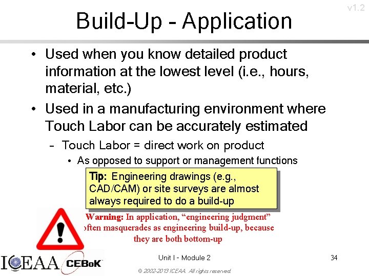
v 1. 2 Build-Up - Application • Used when you know detailed product information at the lowest level (i. e. , hours, material, etc. ) • Used in a manufacturing environment where Touch Labor can be accurately estimated – Touch Labor = direct work on product • As opposed to support or management functions Tip: Engineering drawings (e. g. , CAD/CAM) or site surveys are almost always required to do a build-up Warning: In application, “engineering judgment” often masquerades as engineering build-up, because they are both bottom-up Unit I - Module 2 © 2002 -2013 ICEAA. All rights reserved. 34

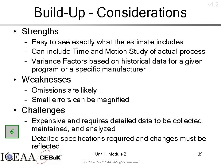
v 1. 2 Build-Up – Considerations • Strengths – Easy to see exactly what the estimate includes – Can include Time and Motion Study of actual process – Variance Factors based on historical data for a given program or a specific manufacturer • Weaknesses – Omissions are likely – Small errors can be magnified • Challenges 6 – Expensive and requires detailed data to be collected, maintained, and analyzed – Detailed specifications required and changes must be reflected Unit I - Module 2 © 2002 -2013 ICEAA. All rights reserved. 35

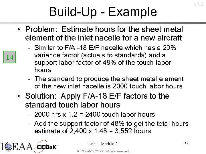
v 1. 2 Build-Up - Example • Problem: Estimate hours for the sheet metal element of the inlet nacelle for a new aircraft 14 – Similar to F/A – 18 E/F nacelle which has a 20% variance factor (actuals to standards) and a support labor factor of 48% of the touch labor hours – The standard to produce the sheet metal element of the new inlet nacelle is 2000 touch labor hours • Solution: Apply F/A-18 E/F factors to the standard touch labor hours – 2000 hrs x 1. 2 = 2400 touch labor hours – Add the support factor of 48% to get the total hours estimate of 2, 400 x 1. 48 = 3, 552 hours Unit I - Module 2 © 2002 -2013 ICEAA. All rights reserved. 36

Build-Up – Uncertainty and Risk • Uncertainty – Uncertainty in Design Specs – Uncertainty in performance to standards (labor) – Uncertainty in unit costs, scrap rates (material) • Risk – Omissions – Historical growth of design specs – Difficulty of integration Unit I - Module 2 © 2002 -2013 ICEAA. All rights reserved. 37 v 1. 2

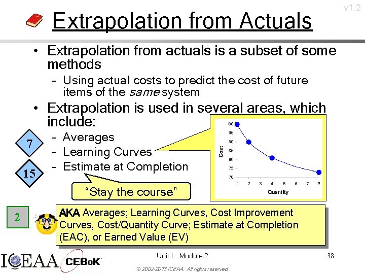
v 1. 2 Extrapolation from Actuals • Extrapolation from actuals is a subset of some methods – Using actual costs to predict the cost of future items of the same system • Extrapolation is used in several areas, which include: 7 15 – Averages – Learning Curves – Estimate at Completion “Stay the course” 2 AKA Averages; Learning Curves, Cost Improvement Curves, Cost/Quantity Curve; Estimate at Completion (EAC), or Earned Value (EV) Unit I - Module 2 © 2002 -2013 ICEAA. All rights reserved. 38

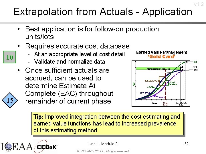
Extrapolation from Actuals - Application v 1. 2 • Best application is for follow-on production units/lots • Requires accurate cost database 10 Earned Value Management – At an appropriate level of cost detail – Validate and normalize data • Once sufficient actuals are accrued, can be used to determine Estimate At Complete (EAC) throughout 15 remainder of current phase ‘Gold Card’ EAC TAB Management Reserve BAC PMB Schedule Variance $ Cost Variance ACWP BCWS BCWP time Time Now Completion Date Tip: Improved integration between the cost estimating and earned value functions has lead to increased prevalence of this estimating method Unit I - Module 2 © 2002 -2013 ICEAA. All rights reserved. 39

Extrapolation from Actuals – Considerations v 1. 2 • Strengths – – Utilizes actual costs to predict future costs Can be applied to hours, materials, total costs Highest credibility and greatest accuracy when properly applied Many government bodies require or encourage the use of this technique • Weaknesses: – Work to date may not be representative of work to go – Extrapolating beyond a reasonable range • Challenges: – – Unknown events affecting bookkeeping of actuals Changes in cost accounting methods Contract changes affecting actuals Configuration changes, process changes all have impacts Unit I - Module 2 © 2002 -2013 ICEAA. All rights reserved. 40

Extrapolation from Actuals – Uncertainty and Risk • Uncertainty – Uncertainty in Learning Curve – Uncertainty in EAC v 1. 2 7 15 • Risk – Insufficient cost history – Cost history not representative of future work – Unrealistic baselines, excessive optimism, and the EAC “tail chase” “Do Not Sum Earned-Value-Based WBS-Element Estimates-at-Completion”, S. A. Book, SCEA National Conference and Training Workshop, 2000 Unit I - Module 2 © 2002 -2013 ICEAA. All rights reserved. 41

v 1. 2 Expert Opinion Unit I - Module 2 © 2002 -2013 ICEAA.

v 1. 2 Expert Opinion - Method • Uses an expert or a group of experts to estimate the cost of a system 1 17 – One-on-one interviews – Round-table discussions – Delphi Technique AKA Engineering Judgment, Round Table, Delphi Technique Tip: Expert Opinion refers to direct assessment of costs. Expert judgment is expected to be applied in any of the previously-described legitimate cost estimating techniques. Unit I - Module 2 © 2002 -2013 ICEAA. All rights reserved. Warning: Expert Opinion alone is not widely considered to be a valid technique 43

v 1. 2 Expert Opinion - Application • Only used when more objective techniques are not applicable • Used to corroborate or adjust objective data – Cross check historical based estimate • Use for high-level, low-fidelity estimating (e. g. , sanity check) Tip: Expert Opinion is the least regarded • Last resort and most dangerous method, but it is seductively easy. Most lexicons do not even admit it as a technique, but it is included here for completeness. Unit I - Module 2 © 2002 -2013 ICEAA. All rights reserved. 44

Expert Opinion – Considerations v 1. 2 • Strengths – Good cross check of other estimate from Subject Matter Expert (SME) point of view – Provides expert perspective that facilitates understanding • Weaknesses 8 – Completely subjective without use of other techniques – Low-to-nil credibility – Difficult to run risk around an expert opinion Tip: It is preferable to find data to support a credible basis, which may jibe with the expert-based estimate if it is implicitly founded on the same data Unit I - Module 2 © 2002 -2013 ICEAA. All rights reserved. 45

Expert Opinion – Uncertainty and Risk v 1. 2 • Uncertainty – Human tendency to (significantly) understate error bands • Risk – Faulty recollection of “anecdotal actuals” – Gaming – Excessive optimism (or conservatism) Unit I - Module 2 © 2002 -2013 ICEAA. All rights reserved. 46

v 1. 2 Using Cost Estimating Techniques • Estimate Requirements • Top Down vs. Bottom Up • Cost Element Structure (CES) • Technique Selection • Checking Results • Documentation Unit I - Module 2 © 2002 -2013 ICEAA. All rights reserved. 47

v 1. 2 Estimate Requirements • Why are we developing this estimate? What will it be used for? – Milestone A, B, or C decision – Developing a budget – Developing a “ballpark” or rough order of magnitude (ROM) estimate – Comparing alternatives – Developing or evaluating proposals Unit I - Module 2 © 2002 -2013 ICEAA. All rights reserved. 48

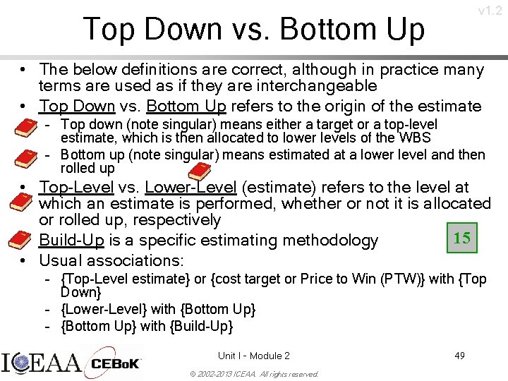
v 1. 2 Top Down vs. Bottom Up • The below definitions are correct, although in practice many terms are used as if they are interchangeable • Top Down vs. Bottom Up refers to the origin of the estimate – Top down (note singular) means either a target or a top-level estimate, which is then allocated to lower levels of the WBS – Bottom up (note singular) means estimated at a lower level and then rolled up • Top-Level vs. Lower-Level (estimate) refers to the level at which an estimate is performed, whether or not it is allocated or rolled up, respectively 15 • Build-Up is a specific estimating methodology • Usual associations: – {Top-Level estimate} or {cost target or Price to Win (PTW)} with {Top Down} – {Lower-Level} with {Bottom Up} – {Bottom Up} with {Build-Up} Unit I - Module 2 © 2002 -2013 ICEAA. All rights reserved. 49

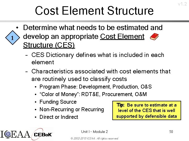
v 1. 2 Cost Element Structure • Determine what needs to be estimated and 1 develop an appropriate Cost Element Structure (CES) – CES Dictionary defines what is included in each element – Characteristics associated with cost elements that are routinely used to classify costs • • • Program Phase: Development, Production, O&S “Color of Money”: RDT&E, Procurement, O&M Funding Source Tip: Be sure to estimate at a Non-Recurring or Recurring level of the CES that is well supported by defensible data Direct or Indirect Unit I - Module 2 © 2002 -2013 ICEAA. All rights reserved. 50

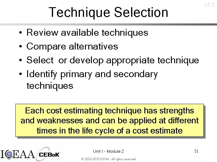
v 1. 2 Technique Selection • • Review available techniques Compare alternatives Select or develop appropriate technique Identify primary and secondary techniques Each cost estimating technique has strengths and weaknesses and can be applied at different times in the life cycle of a cost estimate Unit I - Module 2 © 2002 -2013 ICEAA. All rights reserved. 51

v 1. 2 Checking Results • Cross Checking your results greatly increases credibility 16 – Example: A parametric-based estimate can also show an analogy as a “reasonableness test” – Doesn’t necessarily result in the exact same number, but should be a similar number (same order of magnitude) • An independent* estimate is more detailed than a cross check and attempts to get the same result using a different technique – Example: Use the results from one commercial software estimating package to validate the results of another *Note: “Independent” has many meanings. The most stringent meaning is in Title 10 USC Section 2434 and involves an organization out of the chain of command of the acquiring agency. A looser meaning is an estimate done by an organization unbeholden to the program manager in funding or accountability. The loosest meaning is a separate estimate. Unit I - Module 2 © 2002 -2013 ICEAA. All rights reserved. 52

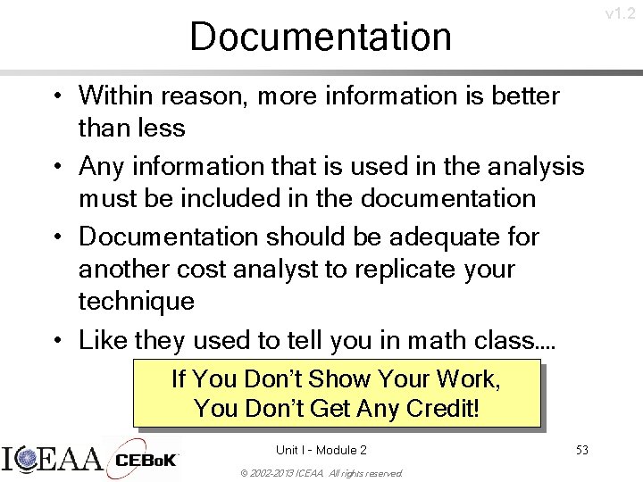
v 1. 2 Documentation • Within reason, more information is better than less • Any information that is used in the analysis must be included in the documentation • Documentation should be adequate for another cost analyst to replicate your technique • Like they used to tell you in math class…. If You Don’t Show Your Work, You Don’t Get Any Credit! Unit I - Module 2 © 2002 -2013 ICEAA. All rights reserved. 53

v 1. 2 Comparison of Techniques Unit I - Module 2 © 2002 -2013

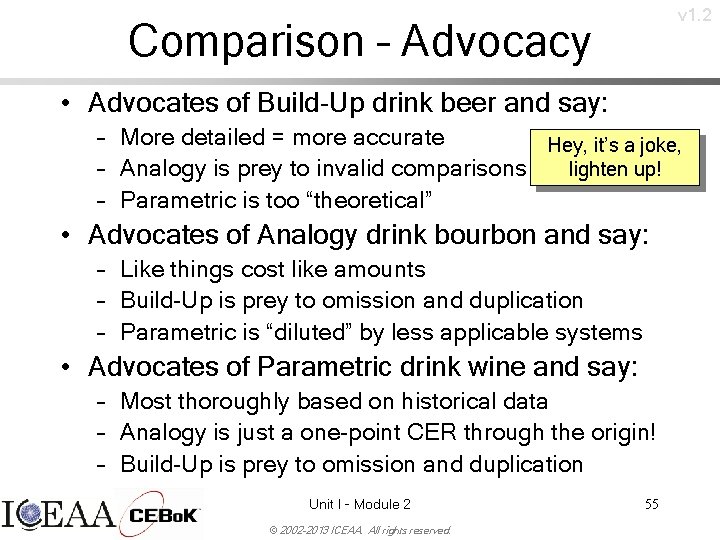
v 1. 2 Comparison – Advocacy • Advocates of Build-Up drink beer and say: – More detailed = more accurate Hey, it’s a joke, lighten up! – Analogy is prey to invalid comparisons – Parametric is too “theoretical” • Advocates of Analogy drink bourbon and say: – Like things cost like amounts – Build-Up is prey to omission and duplication – Parametric is “diluted” by less applicable systems • Advocates of Parametric drink wine and say: – Most thoroughly based on historical data – Analogy is just a one-point CER through the origin! – Build-Up is prey to omission and duplication Unit I - Module 2 © 2002 -2013 ICEAA. All rights reserved. 55

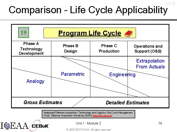
v 1. 2 Comparison – Life Cycle Applicability Program Life Cycle 19 Phase A Technology Development Phase B Design Phase C Production Operations and Support (O&S) Extrapolation From Actuals Parametric Engineering Analogy Gross Estimates Detailed Estimates Integrated Defense Acquisition, Technology and Logistics Life Cycle Management Chart, Defense Acquisition University (DAU), https: //ilc. dau. mil/. Unit I - Module 2 © 2002 -2013 ICEAA. All rights reserved. 56

Cost Estimating Techniques Summary • You need to have all the cost estimating techniques in your repertoire • For each, you need to know: 20 – – – What it is When to apply How to execute Strengths and Weaknesses Challenges The supporting data required Unit I - Module 2 © 2002 -2013 ICEAA. All rights reserved. 57 v 1. 2

v 1. 2 Resources • Integrated Defense Acquisition, Technology, and Logistics Life Cycle Management chart, Defense Acquisition University (DAU) – https: //ilc. dau. mil/ • International Society of Parametric Analysts (ISPA), Parametric Estimating Handbook, 4 th Edition, April 2008 – https: //www. iceaaonline. org/documentation/files/ISPA_PEH_4 th_ed_Final. pdf Unit I - Module 2 © 2002 -2013 ICEAA. All rights reserved. 58

v 1. 2 Related and Advanced Topics • • Analogies and Rates Below-The-Line (BTL) Factors Schedule Estimating Operations and Support (O&S) estimating Unit I - Module 2 © 2002 -2013 ICEAA. All rights reserved. 59

v 1. 2 Analogies and Rates • Analogy scaling can be expressed as a rate – Such rates are common in certain circles • $/lb, mhrs/ton, mhrs/LOC, etc. • Reciprocal = productivity (e. g. , LOC/mhr) • Mathematically equivalent: – $5. 2 M/12, 000 lbs = $433/lb of thrust – $433/lb x 16, 000 lbs = $6. 9 M • Same concerns as with adjusted analogy – Prefer regression-based CER, when possible Unit I - Module 2 © 2002 -2013 ICEAA. All rights reserved. 60

Below-The-Line (BTL) Factors • Typically Systems Engineering, Integration and Test, and Program Management (SEITPM) AKA “Cost-on. Cost” CERs • Often a function of Prime Mission Equipment (PME) 3 • Beware non-statistically-based factors • Similar in application to burdens like Overhead and G&A, but less “deterministic” • Should be modeled using Functional 9 Correlation in the risk model Unit I - Module 2 © 2002 -2013 ICEAA. All rights reserved. 61 v 1. 2

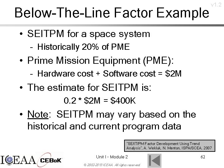
Below-The-Line Factor Example v 1. 2 • SEITPM for a space system – Historically 20% of PME • Prime Mission Equipment (PME): – Hardware cost + Software cost = $2 M • The estimate for SEITPM is: 0. 2 * $2 M = $400 K • Note: SEITPM may vary based on the historical and current program data “SE/IT/PM Factor Development Using Trend Analysis”, A. Wekluk, N. Menton, ISPA/SCEA, 2007 Unit I - Module 2 © 2002 -2013 ICEAA. All rights reserved. 62

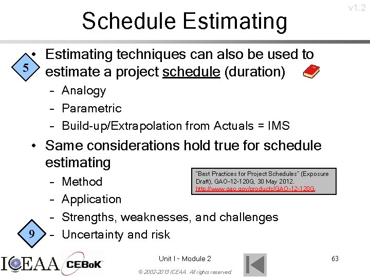
v 1. 2 Schedule Estimating • Estimating techniques can also be used to 5 estimate a project schedule (duration) – Analogy – Parametric – Build-up/Extrapolation from Actuals = IMS • Same considerations hold true for schedule estimating 9 – – “Best Practices for Project Schedules” (Exposure Draft), GAO-12 -120 G, 30 May 2012. http: //www. gao. gov/products/GAO-12 -120 G. Method Application Strengths, weaknesses, and challenges Uncertainty and risk Unit I - Module 2 © 2002 -2013 ICEAA. All rights reserved. 63

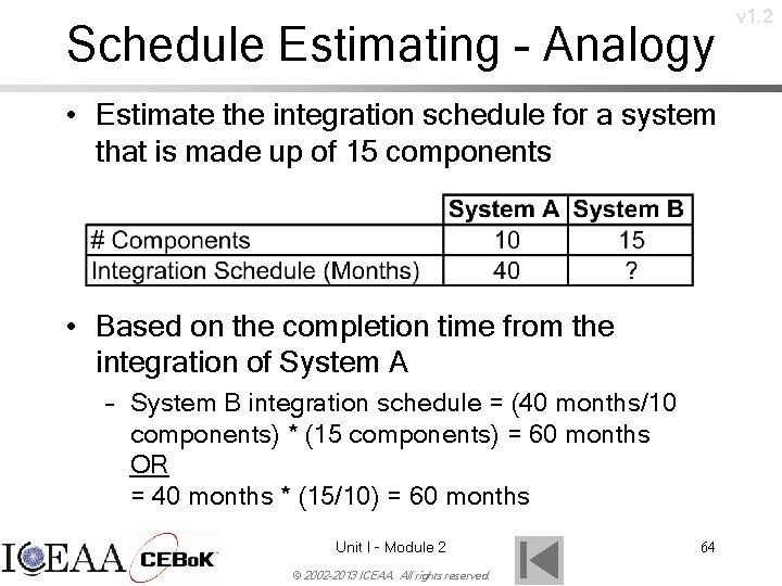
Schedule Estimating - Analogy • Estimate the integration schedule for a system that is made up of 15 components • Based on the completion time from the integration of System A – System B integration schedule = (40 months/10 components) * (15 components) = 60 months OR = 40 months * (15/10) = 60 months Unit I - Module 2 © 2002 -2013 ICEAA. All rights reserved. 64 v 1. 2

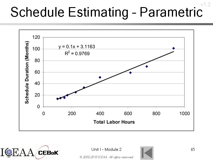
v 1. 2 Schedule Estimating – Parametric Unit I - Module 2 © 2002

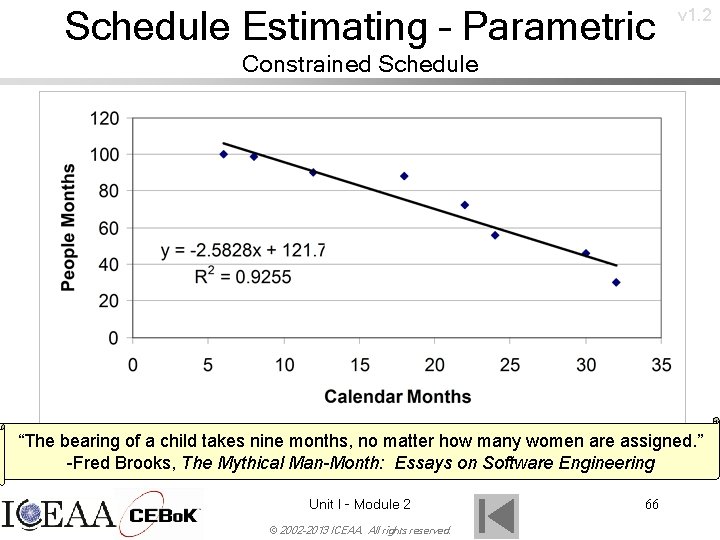
Schedule Estimating – Parametric v 1. 2 Constrained Schedule “The bearing of a child takes nine months, no matter how many women are assigned. ” -Fred Brooks, The Mythical Man-Month: Essays on Software Engineering Unit I - Module 2 © 2002 -2013 ICEAA. All rights reserved. 66

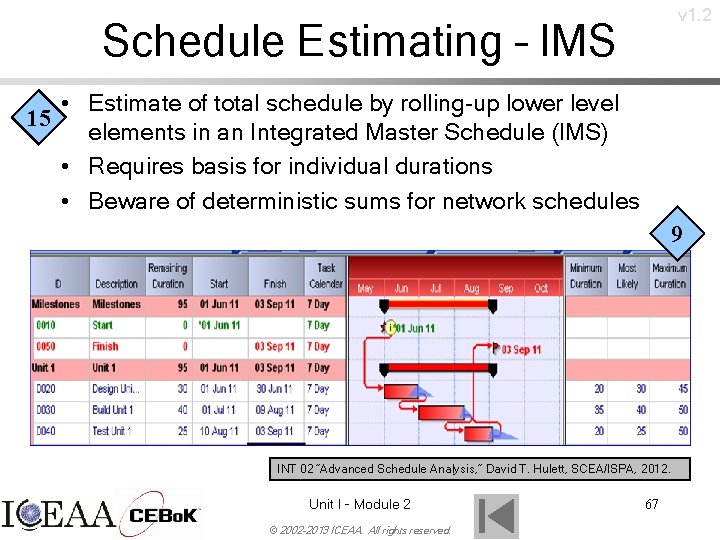
v 1. 2 Schedule Estimating – IMS • Estimate of total schedule by rolling-up lower level 15 elements in an Integrated Master Schedule (IMS) • Requires basis for individual durations • Beware of deterministic sums for network schedules 9 INT 02 “Advanced Schedule Analysis, ” David T. Hulett, SCEA/ISPA, 2012. Unit I - Module 2 © 2002 -2013 ICEAA. All rights reserved. 67

Operations and Support (O&S) Cost Estimating v 1. 2 • Operations and Support (O&S) costs normally make up a large portion of system life cycle costs and are often overlooked • O&S costs are defined as all of the costs associated with operating, maintaining, and supporting a system • O&S costs include costs for: – Personnel – Consumable and repairable materials – Organizational, intermediate, and depot maintenance • Hardware and Software – Facilities – Sustainment AKA Operating and Support (O&S), Operations and Sustainment (O&S), Operations and Maintenance (O&M) Do. D Operating and Support Cost Estimating Guide, OSD CAIG [sic], October, 2007. https: //acc. dau. mil/Community. Browser. aspx? id=187960. Unit I - Module 2 © 2002 -2013 ICEAA. All rights reserved. 68

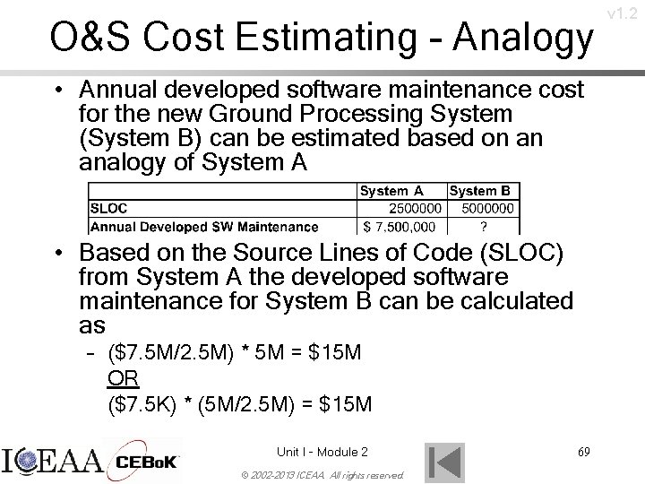
O&S Cost Estimating - Analogy • Annual developed software maintenance cost for the new Ground Processing System (System B) can be estimated based on an analogy of System A • Based on the Source Lines of Code (SLOC) from System A the developed software maintenance for System B can be calculated as – ($7. 5 M/2. 5 M) * 5 M = $15 M OR ($7. 5 K) * (5 M/2. 5 M) = $15 M Unit I - Module 2 © 2002 -2013 ICEAA. All rights reserved. 69 v 1. 2

O&S Cost Estimating - Parametric v 1. 2 3 “How Age Affects Operations and Support Costs Differently Across Platforms, ” S. Grinnell, J. Summerville, R. Coleman , SCEA, 2006. Unit I - Module 2 © 2002 -2013 ICEAA. All rights reserved. “O&S Physics Based Modeling, ” Kevin Cincotta, Do. DCAS, 2006. 70

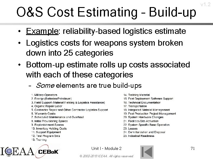
O&S Cost Estimating – Build-up • Example: reliability-based logistics estimate • Logistics costs for weapons system broken down into 25 categories • Bottom-up estimate rolls up costs associated with each of these categories – Some elements are true build-ups Unit I - Module 2 © 2002 -2013 ICEAA. All rights reserved. 71 v 1. 2