Cosmology the Big Bang AY 16 Lecture 19

Cosmology & the Big Bang AY 16 Lecture 19, April 10, 2008 Introduction to Cosmology Basic Principles Fundamental Observations The FRW Metric

“My husband adheres to the Big Bang theory of creation. ”

COSMOLOGY The BIG Picture! The cosmological model dominates much of extragalactic astronomy, in fact much of astronomy & astrophysics, even physics. What is Cosmology? “The study of the large scale structure & evolution of the Universe” What is Cosmogony? “The study of the origin of observable structures” Cosmology is perhaps the oldest real science. Its tied to our “World View. ”

Changing Worldviews Age Universe -----------------------------------------10, 000 years BC --- The Valley you lived in 1, 000 years BC --- Your Kingdom 300 years BC --- The Mediterranean (for Egypto-Greco-Romans, at least!) 100 years AD --- The Earth + Celestial Sphere 400 years ago --- The Solar System 100 years ago --- The Milky Way 75 years ago --- The “Modern” Universe (2 Billion Light -Years in *radius*) Today --- An Infinite Universe (the visible part has a Radius of ~15 Gly)

A Brief History of Extragalactic Astronomy: ~ 1750 Early Rumblings of “Island Universes” from I. Kant, T. Wright, P. Laplace. This seems to have been forgotten soon after. 1800’s Catalogs of Things but no understanding. de la Caille, Messier, Herschel 3, Dreyer William, Caroline & John ~ 1875 The Discovery of the Galaxy --- Kapteyn’s Universe

1910 Removal of the Solar-Centric view 1900 -1920 Shapley and the Great Debate 1907 Bohlin --- M 31 Parallax 1918 Van Maanen --- M 31 Parallax 1885 S Andromeda = SN 1885 a large reflectors + photographic plates 1920 The Shapley-Curtis debate Shapley + Globular Clusters + Cepheids 1924 Hubble & the Hooker --- NGC 6822 Cepheids, eventually M 31 Cepheids

1910 -1930 Theory! Einstein, Friedmann, de. Sitter, Lemaitre, Tolman, Robertson … 1922 Opik’s M 31 Mass-to-Light ratio L = 4πr 2 GMm/r = ½ mv 2 M = ½ v 2 r/G, v 2 1 1 so M/L = ½ G 4πD and Opik estimated D of M 31 at 450 kpc.

1929 Hubble (+Slipher) Velocity-Distance Law 1930’s Hubble’s Classification Scheme for Galaxies (Tuning Fork Diagram) N. B. Absolutely necessary but wrong interpretation, set galaxy evolution back 20 years! Hubble’s Galaxy Counts (Humason) 1937 Zwicky & Smith DARK MATTER 1940’s Galactic Dust, Stellar Populations, Hubble Diagram

1948 Gamow & the Hot Big Bang 1950’s de. Vaucouleurs’ Local “Supergalaxy” Rubin: Flows Dicke: CM HMS Velocities + Hubble Diagram Baade & Sandage: H 0 revisions Minkowski: Radio galaxies 1960’s The Hubble Constant Debate Tinsley: Stellar Evolution Galaxy Evolution

Greenstein & Schmidt: Quasars Arp: Peculiar Galaxies Spinrad &Taylor : Population Synthesis Page: Galaxy Masses 1970’s Stability & Halos Starbursts H 0!!! q 0!!! First Feeble Redshift Surveys CMB Dipole

Galaxy Clusters & X-Rays Gravitational Lenses Galaxy Formation 1980’s Large-Scale Structure Large Scale Flows & Cold Dark Matter Galaxy Counts H 0!!!! IRAS & Dusty Starbursts

1990’s COBE: 2. 723 K + fluctuations Biased galaxy Formation Unified AGN Models Λ!!!!! Concordance Cosmology HST and galaxy evolution 2000+ The Cosmic Web Reionization First Light

COSMOLOGY is a modern subject: Today based on Principles & Observables The basic framework for our current view of the Universe rests on ideas and discoveries (mostly) from the early 20 th century. Basics: Einstein’s General Relativity The Copernican Principle

Fundamental Principles: • Cosmological Principle: (a. k. a. the Copernican principle). There is no preferred place in space --- the Universe should look the same from anywhere The Universe is HOMOGENEOUS and ISOTROPIC. we believe this is true to zeroth order (i. e. on large scales, yes, on small scales, no)

A variant of the CP is • The Perfect Cosmological Principle: The Universe is also the same in time. The STEADY STATE Model (XXX it’s demonstrably wrong) • The Anthropic Cosmological Principle: We see the Universe in a preferrred state (time etc. ) --- when Humans can exist.

the ACP is almost the opposite of the PCP. it leads to the Goldilocks Universe: Not too hot, Not too cold Not too dense, Not too empty Not too young, Not too old…. • Relativistic Cosmological Principle: The Laws of Physics are the same everywhere and everywhen. (!!!) absolutely necessary, often assumed and forgotten. (!!!)

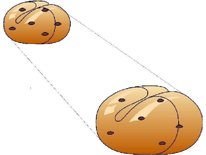
Fundamental Observations: • The Sky is Dark at Night (Olber’s P. ) this implies there must be some limit to the observable Universe. • The Universe is generally Expanding It’s not static. galaxies appear to be moving away from us --- and each other.

Olber’s Paradox

Hubble’s Discovery of Expansion

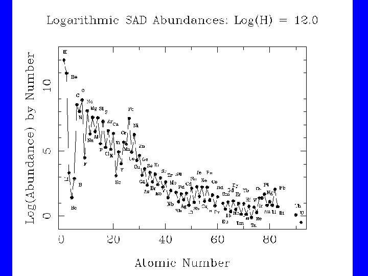
• The Universe is Homogeneous on large scales --- there exists an almost isotropic microwave background (the CMB) of T~3 K a. k. a. relic radiation • The Universe is not Empty. It has stuff in it, stuff consistent with a hot origin (the Universe has a temperature), i. e. contents consistent with nuclear physics operating in an initially hot, dense medium

COBE Fluctuations dt/t < 10 -5, i. e. much smoother than a baby’s bottom!

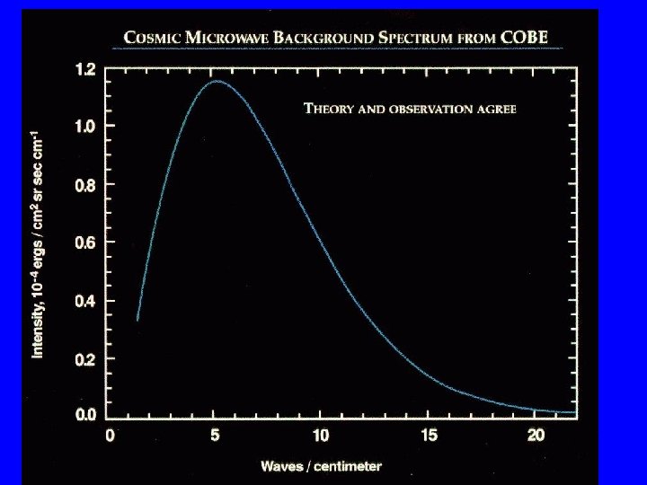
Observational Cosmology consists of taking these bases to build a more detailed picture of the structure and evolution of the Universe. Sometimes to (1) Feed Theorists (2) Kill Theories (3) Explore generally support Gamow’s hot big bang model

COSMOLOGICAL FRAMEWORK: The Friedmann-Robertson-Walker Metric + The Cosmic Microwave Background = THE HOT BIG BANG

The Big Bang WRONG!

WRONG!!!

WRONG ? ? T THE TRUTH BEHIND THE BIG BANG THEORY

How my wife describes my job! RIGHT!

Mathematical Cosmology The simplest questions are Geometric. How is Space measured? Standard 3 -Space Metric: 2 2 ds = dx + dy + dz 2 2 2 = dr + r dθ + r sin θ df In Cartesian or Spherical coordinates in Euclidean Space.

Now make our space Non-Static, but “homogeneous” & “isotropic” 2 2 2 ds = R (t)(dx + dy + dz ) And then allow transformation to a more general geometry (i. e. allow non. Euclidean geometry) but keep isotropic and homogeneous:

2 2 -2 ds = (1+1/4 kr ) 2 2 2 (dx +dy +dz )R (t) 2 2 where r = x + y + z , and k is a measure of space curvature. Note the Special Relativistic Minkowski Metric 2 2 2 ds = c dt – (dx +dy + dz )

So, if we take our general metric and add the 4 th (time) dimension, we have: 2 2 2 2 ds = c dt – R (t)(dx +dy + dz )/(1+kr /4) or in spherical coordinates and simplifying, 2 2 2 ds = c dt – R (t)[dr /(1 -kr ) + 2 2 r (dq +sin q df )] which is the (Friedmann)-Robertson-Walker Metric, a. k. a. FRW

• The FRW metric is the most general, non-static, homogeneous and isotropic metric. It was derived ~1930 by Robertson and Walker. R(t), the Scale Factor, is an unspecified function of time (which is usually assumed to be continuous) and k = 1, 0, or -1 = the Curvature Constant For k = -1 or 0, space is infinite

K = +1 Spherical c < pr K = -1 Hyperbolic c > pr K=0 Flat c = pr

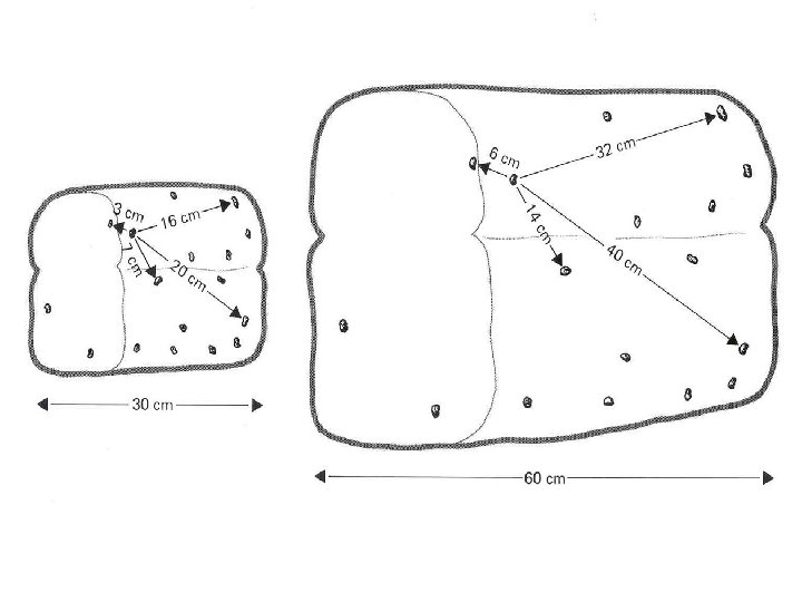
Consider Expansion in an Isotropic Universe l= a l 0 ) t 0 (t l 0 a(t) = Universal Expansion factor

Expansion is self-similar and produces a change in the frequency of received radiation. If t 0 = now, here, observed & t 1 = the time at which light is emitted from a distant object in the scaled universe: a(t)δt R(t)l t 0+Δt 0 R 0 (t) l te+Δte te = t 1

1/Δte = υ1 frequency of emitted radiation υ0 υ1 = a(t 1) a(t 0) = λ 1 λ 0 so υ1, λ 1 = lab or rest frequency/wavelength and υ0, λ 0 = observed frequency/wavelength and if we define z ≡ redshift = R(t 0) a(t 0) Then 1 + z = = R(t 1) a(t 1) λ 0 – λ 1 λ 0

For small z we can interpret this “redshift” in terms of a Doppler shift, cz = v, or Doppler velocity. For small Δt, if r 0 = 0 (set origin to us, the observer), we have: r 1 = c (t 0 - t 1)/R(t 0) d = r 1 R(t 0) = c(t 0 -t 1) the distance and thus 1 d. R(t 1) cz = c(t 0 – t 1) R(t 0) dt

so v = cz = H 0 d d. R(t 0) 1 d. R(t 1) 1 where H 0 = ≈ dt R(t 0) dt R(t 1) is the definition of Hubble’s Constant. Note that this is true for small z only. This formula for distance is NOT subject to special relativity. The convention is to quote apparent velocities as v = cz.

The apparent (radial) velocity of any object is made up of three parts v = v. H + v. P + v. G v. H = the cosmological stretching of the metric, a. k. a. the Hubble Flow v. P = the component of the “peculiar” velocity w. r. t. the Hubble Flow that is an actual space velocity. v. P is Doppler, so computations of dynamical properties like cluster velocity dispersions that result from v. P do require the (1+v 2/c 2) – 1/2 correction. v. G = the gravitational redshift, usually tiny

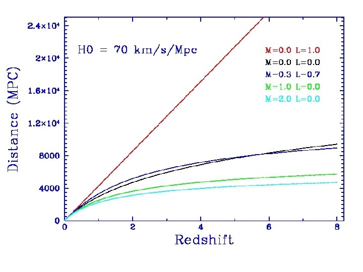
Expansion Age & Hubble Distance The Hubble Constant has units of inverse time; its actually also a measure of the expansion age of the Universe: τH = H 0 -1 = 9. 78 x 109 h-1 years = 3. 09 x 1017 h-1 s where H 0 = 100 h km/s/Mpc And the Hubble Distance is DH = c/H 0 = 3000 h-1 Mpc = 9. 26 x 1025 h-1 m

What about the scale factor R(t)? R(t) is specified by Physics we can use Newtonian Physics (the Newtonian approximation) but now General Relativity holds. Start with Einstein’s (tensor) Field Equations G u = 8 p. T n + Lg u and G u = R n - 1/2 g u R

Where T n is the Stress Energy tensor R n is the Ricci tensor g u is the metric tensor G u is the Einstein tensor and R is the scalar curvature R n - 1/2 g u R = 8 p. T n + Lg u is the Einstein Equation

The vector/scalar terms of the Tensor Field Equations give the linear form Einstein’s Equations: 2 2 2 (d. R/dt) /R + kc /R = 8 p. Ge/3 c +Lc /3 2 energy density 2 2 CC 2 2(d R/dt )/R + (d. R/dt) /R + kc /R = -8 p. GP/c +Lc 3 pressure term 2

And Friedmann’s Equations: 2 2 2 (d. R/dt) = 2 GM/R + Lc R /3 – kc 2 2 Ro [(8 p. G/3)ro – Ho] if L = 0 (no Cosmological Constant) 2 2 kc = or 2 (d. R/dt) /R - 8 p. Gro /3 =Lc /3 – kc which is known as Friedmann’s Equation 2 /R 2

Note that if we assume Λ = 0, we have (d 2 R/dt 2)/R = - 4πG (ρ + 3 P) 3 and in a matter dominated Universe, ρ >> P So we can define a critical density by combining the cosmological equations: 3 ρC = 8πG . 2 3 H 02 R = R 2 8πG

And we define the ratio of the density to the critical density as the parameter Ω ≡ ρ/ρC For a matter dominated, Λ=0 cosmology, Ω > 1 = closed Ω = 1 = flat, just bound Ω < 1 = open There are many possible forms of R(t), especially when Λ and P are reintroduced. Its our job to find the right one!

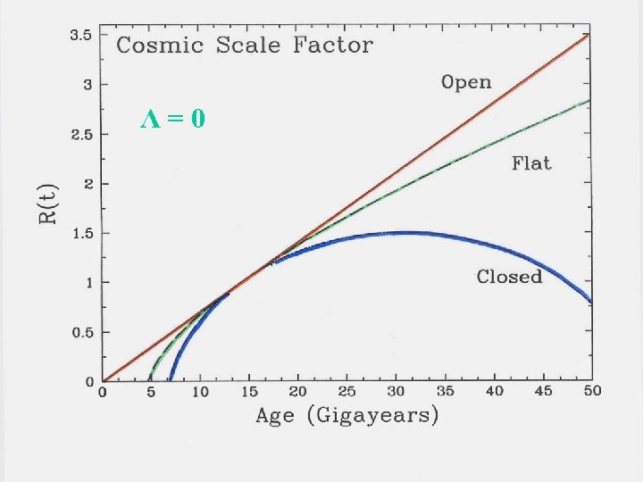
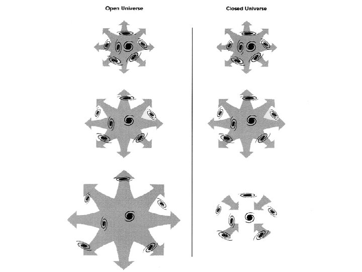
Some of possible forms are: Big Bang Models: Einstein-de. Sitter k=0 flat, open & infinite expands Friedmann-Lemaitre k=-1 hyperbolic “ “ “ k=+1 spherical, closed finite, collapses Leimaitre Λ ≠ 0 k=+1 spherical, closed finite, expands

Non-Big Bang Models Eddington-Lemaitre Λ≠ 0 k=+1 spherical, closed, finite, static then expands Steady State k=0 flat, open, infinite, stationary de. Sitter k=0 empty, no singularity, open, infinite H 02 (Ω 0 – 1) + 1/3 Λ 0 k= c 2 ≡ Radius of Curvature of the Universe

R(t) A Child’s Garden E-L F-L, 0 Ed. S of Cosmological Models SS, d. S L F-L, C t

Harrison’s Classes Geometric: Closed Open Kinematic: Bang Whimper Static Oscillating

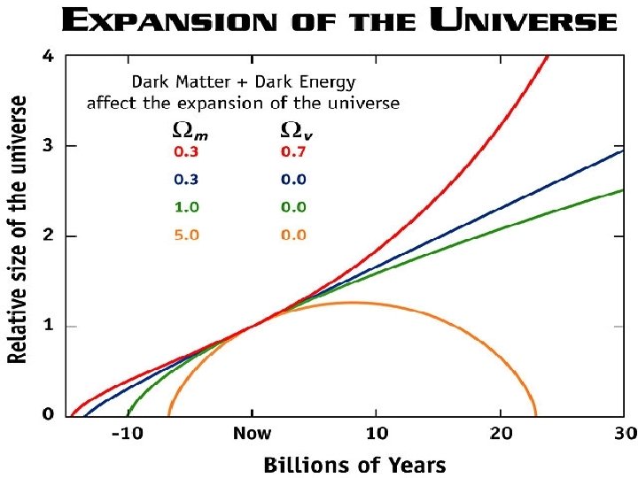
Cosmology is now the search for three numbers: • The Expansion Rate = Hubble’s Constant = H 0 • The Mean Matter Density = Ωmatter • The Cosmological Constant = ΩΛ Taken together, these three numbers describe the geometry of space-time and its evolution. They also give you the Age of the Universe.

The best routes to the first two are in the Nearby Universe: H 0 is determined by measuring distances and redshifts to galaxies. It changes with time in real FRW models so by definition it must be measured locally. W(matter) is determined locally by (1) a census, (2) topography, or (3) gravity versus the velocity field (how things move in the presence of lumps).

The cosmological constant is determined by measuring geometry on large scales --- e. g. by the supernovae Hubble Diagram (distance versus redshift) Or by a difference technique, e. g. CMB shows us that the Universe is Flat, but ΩM is only 0. 3, so ……

Lookback Time For a Friedmann-Lemaitre Big-Bang Model, the lookback time as a function of redshift is τL = H 0 -1 z ( 1+z ) for q 0=0; Λ=0 = 2/3 H 0 -1 [1 – (1 + z)-3/2] for q 0=1/2, Λ=0

Cosmological Age Calculation For models w/o a Cosmological Constant, for q 0 = 0 q 0 = ½ q 0 > ½ where t 0 = H 0 -1 t 0 = (2/3)H 0 t 0 = H 0 -1 -1 (1/(1 -2 q 0) +. . ) q 0 = W/2 (if L = 0)

For the general case (with a CC), the full form is: t 0 = -1 -H 0 ∫ 0 2 (1+z)[(1+z) (Wmz+1) – ∞ -1/2 (WLz(z+2))] dz and a good approximation is t 0 = -1 -1 1/2 (2/3) H 0 sinn [(|1 -Wa|/Wa) ] 1/2 / |[1 -Wa]|

Where Wa = Wmatter -0. 3*Wtotal + 0. 3 and sinn-1 = sinh-1 if = sin-1 if Wa </= 1 Wa > 1 (from Carroll, Press and Turner, 1992) Also, for a flat model with L, t 0 = -1 (2/3)H 0 WL -1/2 ln[(1+WL 1/2 )/(1 -WL) 1/2 ]

Classical Cosmological Tests Use observations to test/measure the cosmological model: Observables: Apparent magnitudes Redshifts Angular Diameters Number Counts Ages of Things (rocks, star clusters)

(1) Magnitude vs Redshift (The Hubble Diagram) (assume or find a standard candle) log cz 1 1/2 0 -1 V magnitude (corrected) q 0

(2) Counts vs Magnitude (Evolution? ) (3) Angular Diameter vs Redshift (Yardstick) (4) Age Consistency (rocks vs expansion age) (5) Density versus Redshift (galaxy evolution again)