Cosmology Lite A brief treatment of some basic

Cosmology Lite A brief treatment of some basic topics in cosmology 1) Overall framework: expansion and three differential relations 2) The Friedman equation and its solutions 3) The angular relations: curved space 4) Space time diagrams 5) Real time cosmology

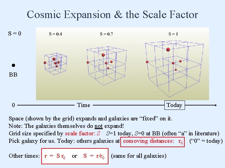
Cosmic Expansion & the Scale Factor S=0 BB 0 Time Today Space (shown by the grid) expands and galaxies are “fixed” on it. Note: The galaxies themselves do not expand! Grid size specified by scale factor: S S=1 today, S=0 at BB (often “a” in literature) Pick galaxy for us. Today: others galaxies at comoving distances: r 0 (“ 0” = today) Other times: r = S r 0 or S = r/r 0 (same for all galaxies)

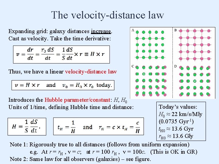
The velocity-distance law Expanding grid: galaxy distances increase. Cast as velocity. Take the time derivative: Thus, we have a linear velocity-distance law Introduces the Hubble parameter/constant: H, H 0 Units of 1/time, defining Hubble time and distance: Today’s values: H 0 ≈ 22 km/s/Mly (0. 0735 Gyr-1) t. H 0 ≈ 13. 6 Gyr r. H 0 ≈ 13. 6 Gly Note 1: Rigorously true to all distances (follows from uniform expansion) e. g. At r = r. H , v = c; at r = 100 r. H , v = 100 c. (This is OK in GR) Note 2: Same law for all observers (galaxies) – see figure.

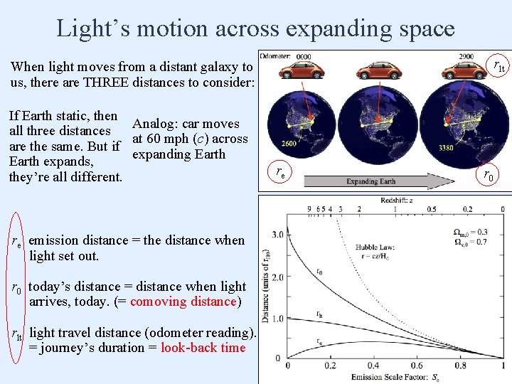
Light’s motion across expanding space rlt When light moves from a distant galaxy to us, there are THREE distances to consider: If Earth static, then Analog: car moves all three distances at 60 mph (c) across are the same. But if expanding Earth expands, they’re all different. re emission distance = the distance when light set out. r 0 today’s distance = distance when light arrives, today. (= comoving distance) rlt light travel distance (odometer reading). = journey’s duration = look-back time re r 0

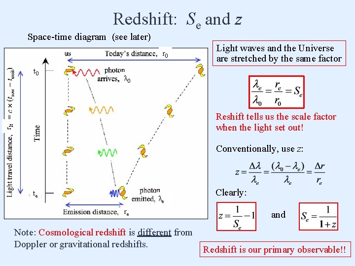
Redshift: Se and z Space-time diagram (see later) r 0 t 0 Light waves and the Universe are stretched by the same factor λ 0 rlt Reshift tells us the scale factor when the light set out! Conventionally, use z: te λe re Note: Cosmological redshift is different from Doppler or gravitational redshifts. Clearly: and Redshift is our primary observable!!

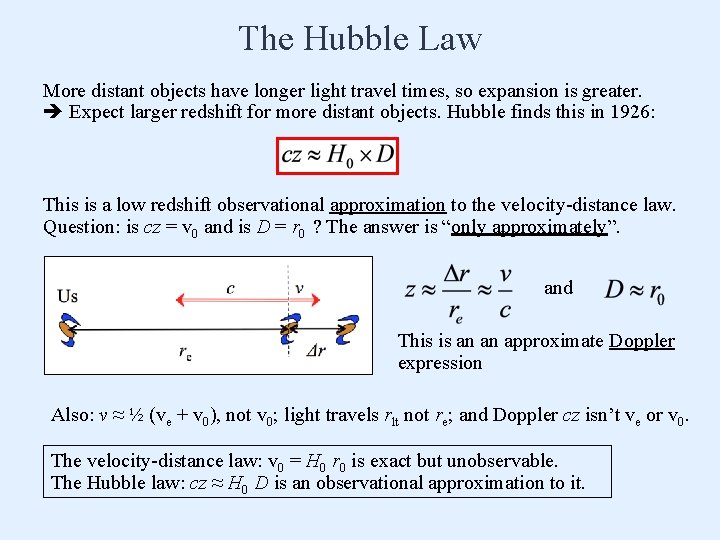
The Hubble Law More distant objects have longer light travel times, so expansion is greater. Expect larger redshift for more distant objects. Hubble finds this in 1926: This is a low redshift observational approximation to the velocity-distance law. Question: is cz = v 0 and is D = r 0 ? The answer is “only approximately”. and This is an an approximate Doppler expression Also: v ≈ ½ (ve + v 0), not v 0; light travels rlt not re; and Doppler cz isn’t ve or v 0. The velocity-distance law: v 0 = H 0 r 0 is exact but unobservable. The Hubble law: cz ≈ H 0 D is an observational approximation to it.

Changing velocities; the velocity factor: V How does a given galaxy’s recession velocity change over time? (Note: velocity-distance law is for a fixed time; different galaxies have v Analogous to scale factor is velocity factor, V: S and V are dimensionless Divide v = dr/dt by v 0 = H 0 r 0 Normalized version of v = dr/dt S(t) and V(t) r)

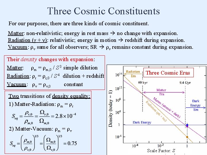
Three Cosmic Constituents For our purposes, there are three kinds of cosmic constituent. Matter: non-relativistic; energy in rest mass no change with expansion. Radiation (γ + ν): relativistic; energy in motion redshift during expansion. Vacuum: ρv same for all observers; SR ρv remains constant during expansion. Their density changes with expansion: Matter: ρm = ρm, 0 / S 3 simple dilution Radiation: ρr = ρr, 0 / S 4 dilution + redshift Vacuum: ρv = ρv, 0 constant Three Cosmic Eras Two transitions of density equality: 1) Matter-Radiation: ρm = ρr 2) Matter-Vacuum: ρm = ρv Scale Factor: S

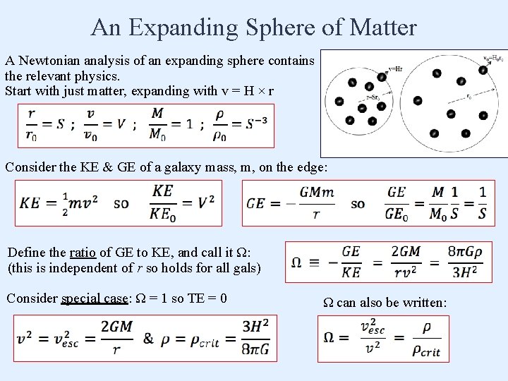
An Expanding Sphere of Matter A Newtonian analysis of an expanding sphere contains the relevant physics. Start with just matter, expanding with v = H × r Consider the KE & GE of a galaxy mass, m, on the edge: Define the ratio of GE to KE, and call it Ω: (this is independent of r so holds for all gals) Consider special case: Ω = 1 so TE = 0 Ω can also be written:

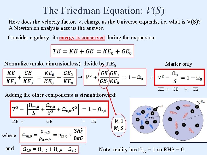
The Friedman Equation: V(S) How does the velocity factor, V, change as the Universe expands, i. e. what is V(S)? A Newtonian analysis gets us the answer. Consider a galaxy: its energy is conserved during the expansion: Normalize (make dimensionless): divide by KE 0 Adding the other components is straightforward: KE + GE = Matter only KE + GE = TE where and Note: reality has Ωt, 0 = 1 so RHS = 0. TE

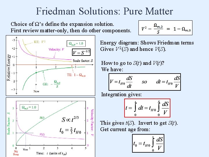
Friedman Solutions: Pure Matter Choice of Ω’s define the expansion solution. First review matter-only, then do other components. Relative Energy diagram: Shows Friedman terms Gives V 2(S) and hence V(S). How to go to S(t) and V(t)? We have: Integration gives: This gives t(S). Invert to get S(t). Get current age from:

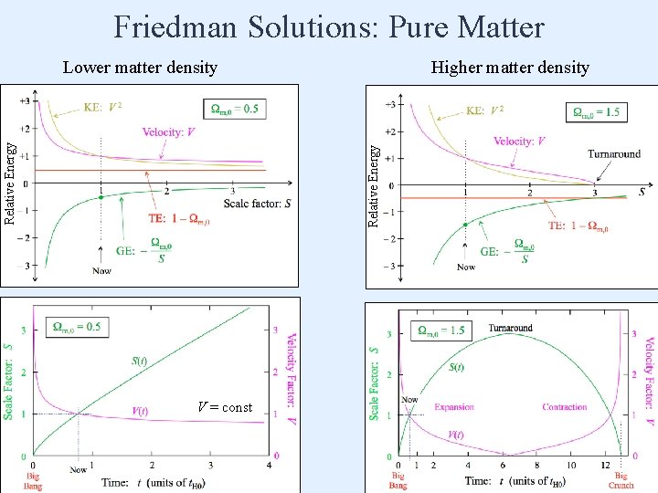
Friedman Solutions: Pure Matter Higher matter density Relative Energy Lower matter density V = const

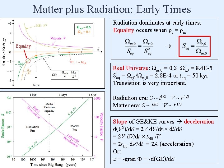
Matter plus Radiation: Early Times Relative Energy Radiation dominates at early times. Equality occurs when ρr = ρm Equality Real Universe: Ωm, 0 = 0. 3 Ωr, 0 = 8. 4 E-5 Seq = Ωr, 0/Ωm, 0 = 2. 8 E-4 or teq = 50 kyr Transistion is very important. Radiation era: S ~ t 1/2 V ~ t-1/2 Matter era: S ~ t 2/3 V ~ t-1/3 Slope of GE&KE curves deceleration d(V 2)/d. S = 2 V d. V/dt × dt/d. S = 2 V d. V/dt × t. H 0 /V = 2 t. H 0 d. V/dt = 2 A (acceleration) Or: a = -grad Φ = -d(GE)/d. S

Relative Energy Vacuum Because vacuum GE gets more negative with S, KE increases with S giving acceleration. For Ωv, 0 = 1, we have V = S. This gives exponential growth with efolding time t. H 0: Note: this is the nature of Inflation, where the vacuum density is very high so t. H 0 is very short.

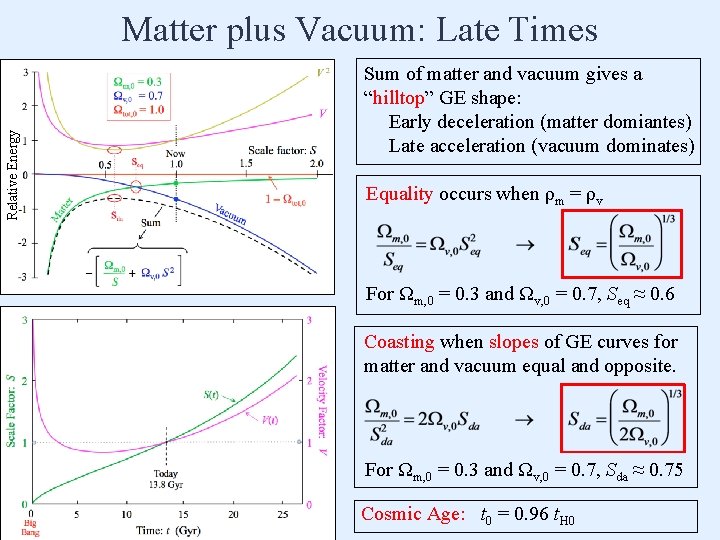
Relative Energy Matter plus Vacuum: Late Times Sum of matter and vacuum gives a “hilltop” GE shape: Early deceleration (matter domiantes) Late acceleration (vacuum dominates) Equality occurs when ρm = ρv For Ωm, 0 = 0. 3 and Ωv, 0 = 0. 7, Seq ≈ 0. 6 Coasting when slopes of GE curves for matter and vacuum equal and opposite. For Ωm, 0 = 0. 3 and Ωv, 0 = 0. 7, Sda ≈ 0. 75 Cosmic Age: t 0 = 0. 96 t. H 0

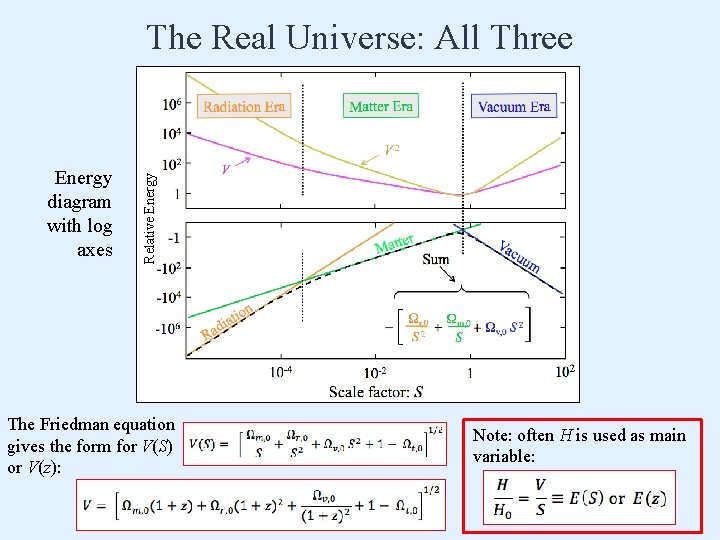
Energy diagram with log axes Relative Energy The Real Universe: All Three The Friedman equation gives the form for V(S) or V(z): Note: often H is used as main variable:

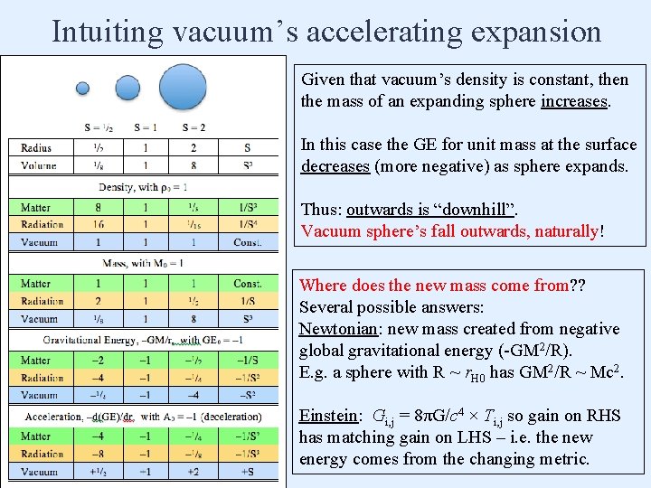
Intuiting vacuum’s accelerating expansion Given that vacuum’s density is constant, then the mass of an expanding sphere increases. In this case the GE for unit mass at the surface decreases (more negative) as sphere expands. Thus: outwards is “downhill”. Vacuum sphere’s fall outwards, naturally! Where does the new mass come from? ? Several possible answers: Newtonian: new mass created from negative global gravitational energy (-GM 2/R). E. g. a sphere with R ~ r. H 0 has GM 2/R ~ Mc 2. Einstein: Gi, j = 8πG/c 4 × Ti, j so gain on RHS has matching gain on LHS – i. e. the new energy comes from the changing metric.

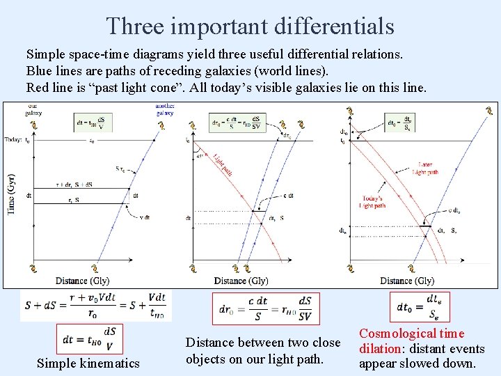
Three important differentials Simple space-time diagrams yield three useful differential relations. Blue lines are paths of receding galaxies (world lines). Red line is “past light cone”. All today’s visible galaxies lie on this line. Simple kinematics Distance between two close objects on our light path. Cosmological time dilation: distant events appear slowed down.

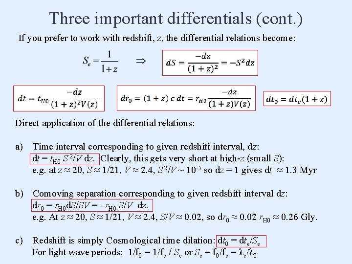
Three important differentials (cont. ) If you prefer to work with redshift, z, the differential relations become: Direct application of the differential relations: a) Time interval corresponding to given redshift interval, dz: dt = t. H 0 S 2/V dz. Clearly, this gets very short at high-z (small S): e. g. at z ≈ 20, S ≈ 1/21, V ≈ 2. 4, S 2/V ~ 10 -5 so dz = 1 gives dt ≈ 1. 3 Myr b) Comoving separation corresponding to given redshift interval dz: dr 0 = r. H 0 d. S/SV = –r. H 0 S/V dz. e. g. At z ≈ 20, S ≈ 1/21, V ≈ 2. 4, S/V ≈ 0. 02, so dr 0 ≈ 0. 02 r. H 0 ≈ 0. 26 Gly. c) Redshift is simply Cosmological time dilation: dt 0 = dte/Se For light wave periods: 1/f 0 = 1/fe / Se or Se = f 0/fe = λe/λ 0

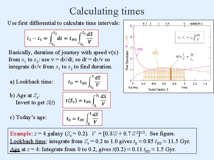
Calculating times Use first differential to calculate time intervals: Basically, duration of journey with speed v(x) from x 1 to x 2: use v = dx/dt, so dt = dx/v so integrate dx/v from x 1 to x 2 to find duration. a) Lookback time: b) Age at Se: Invert to get S(t) c) Today’s age: Example: z = 4 galaxy (Se = 0. 2). V = [0. 3/S + 0. 7 S 2]1/2. See figure. Lookback time: integrate from Se = 0. 2 to 1. 0 gives tlt ≈ 0. 85 t. H 0 ≈ 11. 5 Gyr. Age at z = 4: Integrate from 0 to 0. 2, gives t(0. 2) ≈ 0. 11 t. H 0 ≈ 1. 5 Gyr.

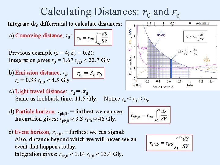
Calculating Distances: r 0 and re Integrate dr 0 differential to calculate distances: a) Comoving distance, r 0: Previous example (z = 4; Se = 0. 2): Integration gives r 0 = 1. 67 r. H 0 ≈ 22. 7 Gly b) Emission distance, re: re = 0. 33 r. H 0 ≈ 4. 5 Gly c) Light travel distance: rlt = ctlt Same as lookback time: 11. 5 Gly. Notice re < rlt < r 0. d) Particle horizon, rph, 0, = furthest we can see: Integration gives: rph, 0 ≈ 3. 3 r. H 0 ≈ 46 Gly. e) Event horizon, reh, 0, = furthest we can signal: Also, distance beyond which we will never see an event that happens today. Integration gives: reh, 0 ≈ 1. 14 r. H 0 ≈ 15. 4 Gly.

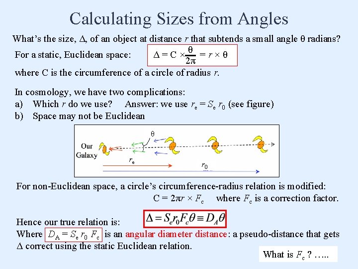
Calculating Sizes from Angles What’s the size, Δ, of an object at distance r that subtends a small angle θ radians? For a static, Euclidean space: Δ=C×θ =r×θ 2π where C is the circumference of a circle of radius r. In cosmology, we have two complications: a) Which r do we use? Answer: we use re = Se r 0 (see figure) b) Space may not be Euclidean θ re r 0 For non-Euclidean space, a circle’s circumference-radius relation is modified: C = 2πr × Fc where Fc is a correction factor. Hence our true relation is: Where DA = Se r 0 Fc is an angular diameter distance: a pseudo-distance that gets Δ correct using the static Euclidean relation. What is Fc ? …. .

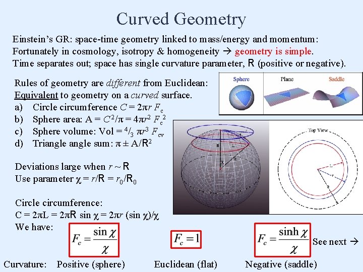
Curved Geometry Einstein’s GR: space-time geometry linked to mass/energy and momentum: Fortunately in cosmology, isotropy & homogeneity geometry is simple. Time separates out; space has single curvature parameter, R (positive or negative). Rules of geometry are different from Euclidean: Equivalent to geometry on a curved surface. a) Circle circumference C = 2πr Fc b) Sphere area: A = C 2/π = 4πr 2 Fc 2 c) Sphere volume: Vol = 4/3 πr 3 Fcv d) Triangle sum: π ± A/R 2 Deviations large when r ~ R Use parameter χ = r/R = r 0/R 0 Circle circumference: C = 2πL = 2πR sin χ = 2πr (sin χ)/χ We have: See next Curvature: Positive (sphere) Euclidean (flat) Negative (saddle)

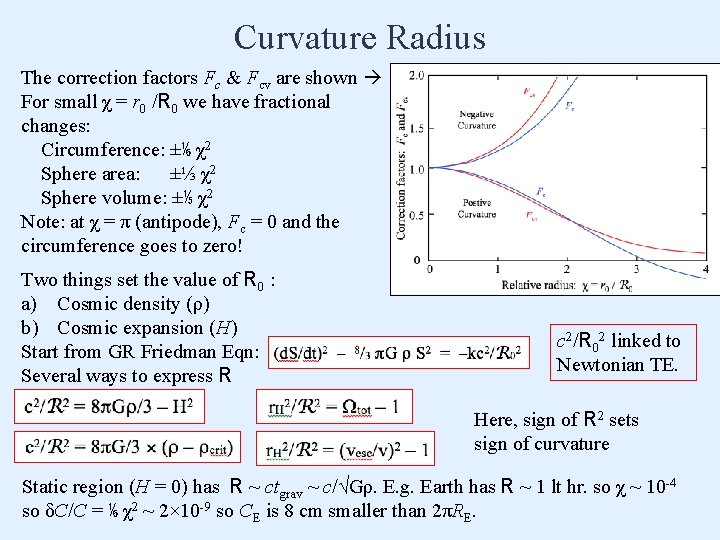
Curvature Radius The correction factors Fc & Fcv are shown For small χ = r 0 /R 0 we have fractional changes: Circumference: ±⅙ χ2 Sphere area: ±⅓ χ2 Sphere volume: ±⅕ χ2 Note: at χ = π (antipode), Fc = 0 and the circumference goes to zero! Two things set the value of R 0 : a) Cosmic density (ρ) b) Cosmic expansion (H) Start from GR Friedman Eqn: Several ways to express R c 2/R 02 linked to Newtonian TE. Here, sign of R 2 sets sign of curvature Static region (H = 0) has R ~ ctgrav ~ c/√Gρ. E. g. Earth has R ~ 1 lt hr. so χ ~ 10 -4 so δC/C = ⅙ χ2 ~ 2× 10 -9 so CE is 8 cm smaller than 2πRE.

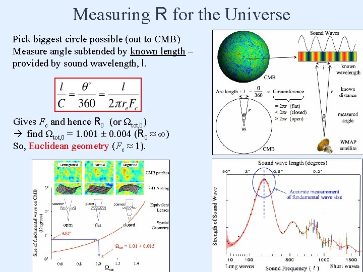
Measuring R for the Universe Pick biggest circle possible (out to CMB) Measure angle subtended by known length – provided by sound wavelength, l. Gives Fc and hence R 0 (or Ωtot, 0) find Ωtot, 0 = 1. 001 ± 0. 004 (R 0 ≈ ∞) So, Euclidean geometry (Fc ≈ 1).

Calculating Luminosity from Flux What’s the Luminosity, L, of an object at distance r with flux f ? For a static, Euclidean space: L = 4π r 2 × f Asph = 4πr 02 Fc 2 Where 4π r 2 = Asph is the area of a sphere of radius r. In cosmology, we have three complications: a) Which r do we use? Answer: we use r 0 b) Space may not be Euclidean: Asph = 4πr 02 Fc 2 c) Redshift reduces photon rate and energy: ×Se-2 Combining these, we have: L = 4π r 02 Fc 2 Se-2 × f We may write this as: L = 4π DL 2 × f where DL = r 0 Fc / Se is the Luminosity Distance: a pseudo-distance that gets L correct using the static Euclidean relation. Note: need extra power of Se (1/Se) for Lλ (Lν) r 0 When the light reaches us, it’s spread over a sphere radius r 0 DL is large: distant galaxies are very faint.

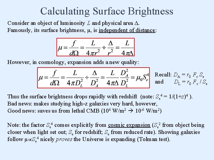
Calculating Surface Brightness Consider an object of luminosity L and physical area Δ. Famously, its surface brightness, μ, is independent of distance: However, in cosmology, expansion adds a new quality: Recall: DA = r 0 Fc Se and DL = r 0 Fc / Se Thus the surface brightness drops rapidly with redshift (note: Se 4 = 1/(1+z)4 ). Bad news: makes studying high-z galaxies very hard, however, Good news: saves us from lethal CMB (106 W/m 2 10 -6 W/m 2) Note: the factor Se 4 comes explicitly from cosmic expansion (Se 2 from object being closer when light set out; Se for redshift; Se from reduced rate). Showing galaxies follow μ Se 4 nicely proves the Universe is expanding (Tolman test).

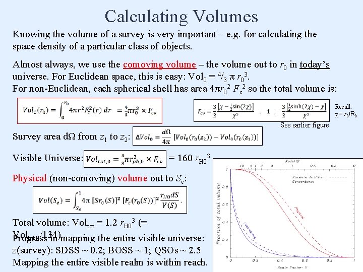
Calculating Volumes Knowing the volume of a survey is very important – e. g. for calculating the space density of a particular class of objects. Almost always, we use the comoving volume – the volume out to r 0 in today’s universe. For Euclidean space, this is easy: Vol 0 = 4/3 π r 03. For non-Euclidean, each spherical shell has area 4πr 02 Fc 2 so the total volume is: Recall: χ = r 0/R 0 See earlier figure Survey area dΩ from z 1 to z 2: Visible Universe: = 160 r. H 03 Physical (non-comoving) volume out to Se: Total volume: Voltot = 1. 2 r. H 03 (= Voltot, 0/134) Progress in mapping the entire visible universe: z(survey): SDSS ~ 0. 2; BOSS ~ 1; QSOs ~ 2. 5 Mapping the entire visible realm is within reach.

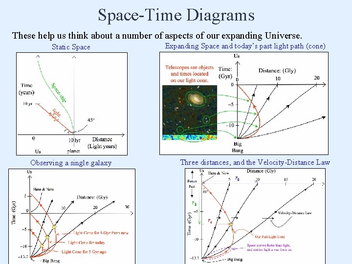
Space-Time Diagrams These help us think about a number of aspects of our expanding Universe. Static Space Observing a single galaxy Expanding Space and today’s past light path (cone) Three distances, and the Velocity-Distance Law r 0 rlt a) Comoving distance, r 0: re

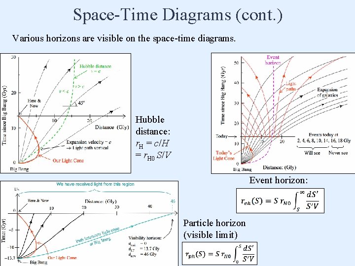
Space-Time Diagrams (cont. ) Various horizons are visible on the space-time diagrams. Hubble distance: r. H = c/H = r. H 0 S/V Event horizon: Particle horizon (visible limit)

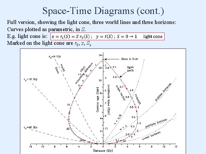
Space-Time Diagrams (cont. ) Full version, showing the light cone, three world lines and three horizons: Curves plotted as parametric, in S. E. g. light cone is: Marked on the light cone are r 0, z, Se

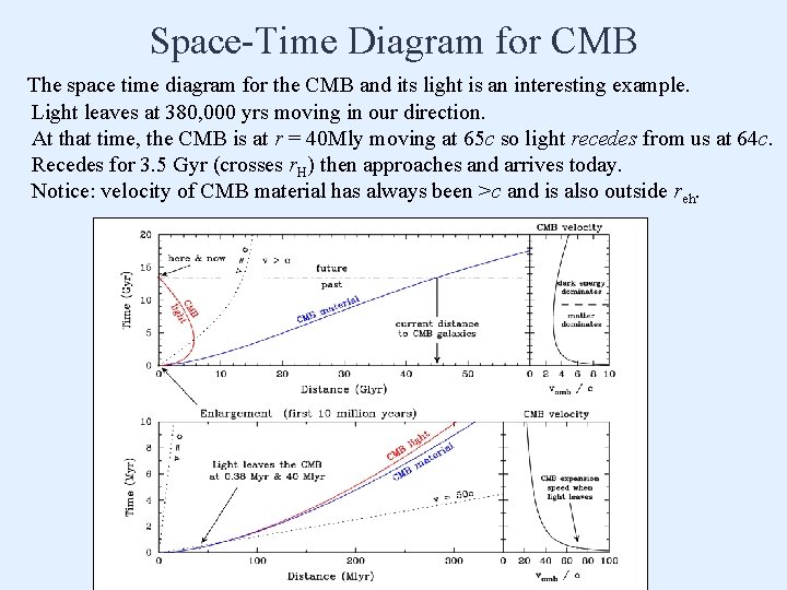
Space-Time Diagram for CMB The space time diagram for the CMB and its light is an interesting example. Light leaves at 380, 000 yrs moving in our direction. At that time, the CMB is at r = 40 Mly moving at 65 c so light recedes from us at 64 c. Recedes for 3. 5 Gyr (crosses r. H) then approaches and arrives today. Notice: velocity of CMB material has always been >c and is also outside reh.

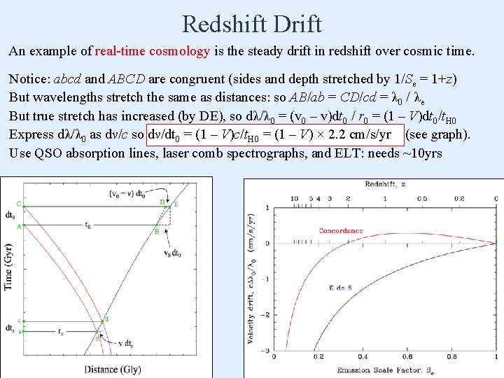
Redshift Drift An example of real-time cosmology is the steady drift in redshift over cosmic time. Notice: abcd and ABCD are congruent (sides and depth stretched by 1/Se = 1+z) But wavelengths stretch the same as distances: so AB/ab = CD/cd = λ 0 / λe But true stretch has increased (by DE), so dλ/λ 0 = (v 0 – v)dt 0 / r 0 = (1 – V)dt 0/t. H 0 Express dλ/λ 0 as dv/c so dv/dt 0 = (1 – V)c/t. H 0 = (1 – V) × 2. 2 cm/s/yr (see graph). Use QSO absorption lines, laser comb spectrographs, and ELT: needs ~10 yrs

End of Cosmology Lite