Cosmology lect 5 Curved Cosmos Observational Cosmology Einstein

Cosmology, lect. 5 Curved Cosmos & Observational Cosmology

Einstein Field Equation

Cosmological Principle

General Relativity A crucial aspect of any particular configuration is the geometry of spacetime: because Einstein’s General Relativity is a metric theory, knowledge of the geometry is essential. Einstein Field Equations are notoriously complex, essentially 10 equations. Solving them for general situations is almost impossible. However, there are some special circumstances that do allow a full solution. The simplest one is also the one that describes our Universe. It is encapsulated in the Cosmological Principle On the basis of this principle, we can constrain the geometry of the Universe and hence find its dynamical evolution.

Cosmological Principle: the Universe Simple & Smooth “God is an infinite sphere whose centre is everywhere and its circumference nowhere” Empedocles, 5 th cent BC Cosmological Principle: Describes the symmetries in global appearance of the Universe: ● Homogeneous The Universe is the same everywhere: - physical quantities (density, T, p, …) ● Isotropic The Universe looks the same in every direction ● Universality Physical Laws same everywhere ● Uniformly Expanding The Universe “grows” with same rate in - every direction - at every location ”all places in the Universe are alike’’ Einstein, 1931

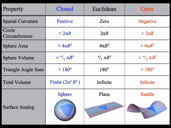
Geometry of the Universe Fundamental Tenet of (Non-Euclidian = Riemannian) Geometry There exist no more than THREE uniform spaces: 1) Euclidian (flat) Geometry Euclides 2) Hyperbolic Geometry Gauß, Lobachevski, Bolyai 3) Spherical Geometry Riemann uniform= homogeneous & isotropic (cosmological principle)

Curvature of the Universe: Robertson-Walker Metric

Spherical Surface Distances

Spherical Surface Distances: alternative – geodetic distance x

Spherical Space Distances Spherical surface is a 2 -D section through an isotropic curved 3 D space: generalization to 3 D solid angle (θ, φ)

Spherical Space Distances alternative: geodetic distance

Minkowski Metric spherically isotropic 3 D space

Robertson-Walker Metric Distances in a uniformly curved spacetime is specified in terms of the Robertson-Walker metric. The spacetime distance of a point at coordinate (r, θ, φ) is: where the function Sk(r/Rc) specifies the effect of curvature on the distances between points in spacetime

Conformal Time

Conformal Time Proper time τ metric Conformal Time η(t) Robertson-Walker

Observational Cosmology in FRW Universe

Redshift

Cosmic Redshift

Cosmic Time Dilation

Cosmic Time Dilation In an (expanding) space with Robertson-Walker metric, In a RW metric, light travels with Cosmic Time Dilation:

Cosmic Time Dilation In Evidence Cosmic Time Dilation: light curves supernovae (exploding stars): characteristic time interval over which the supernova rises and then dims: systematic shift with redshift (depth)

Hubble Expansion

Expanding Universe • Einstein, de Sitter, Friedmann and Lemaitre all realized that in General Relativity, there cannot be a stable and static Universe: • The Universe either expands, or it contracts … • Expansion Universe encapsulated in a GLOBAL expansion factor a(t) • All distances/dimensions of objects uniformly increase by a(t): at time t, the distance between two objects i and j has increased to • Note: by definition we chose a(t 0)=1, i. e. the present-day expansion factor

Interpreting Hubble Expansion • Cosmic Expansion manifests itself in the in a recession velocity which linearly increases with distance • this is the same for any galaxy within the Universe ! • There is no centre of the Universe: would be in conflict with the Cosmological Principle

Hubble Expansion · Cosmic Expansion is a uniform expansion of space · Objects do not move themselves: they are like beacons tied to a uniformly expanding sheet:

Hubble Expansion · Cosmic Expansion is a uniform expansion of space · Objects do not move themselves: Comoving Position they are like beacons tied to a uniformly expanding sheet: Hubble Parameter: Comoving Position Hubble “constant”: H 0� H(t=t 0)

Hubble Parameter · For a long time, the correct value of the Hubble constant H 0 was a major unsettled issue: H 0 = 50 km s-1 Mpc-1 H 0 = 100 km s-1 Mpc-1 · This meant distances and timescales in the Universe had to deal with uncertainties of a factor 2 !!! · Following major programs, such as Hubble Key Project, the Supernova key projects and the WMAP CMB measurements,

Hubble Expansion Edwin Hubble (1889 -1953) v=H r Hubble Expansion

Hubble Parameter · For a long time, the correct value of the Hubble constant H 0 was a major unsettled issue: H 0 = 50 km s-1 Mpc-1 H 0 = 100 km s-1 Mpc-1 · This meant distances and timescales in the Universe had to deal with uncertainties of a factor 2 !!! · Following major programs, such as Hubble Key Project, the Supernova key projects and the WMAP CMB measurements,

Hubble Expansion Space expands: displacement - distance Hubble law: velocity - distance

Deformation Nonlinear Descriptions Cosmic Volume Element The evolution of a fluid element on its path through space may be specified by its velocity gradient: in which θ: velocity divergence contraction/expansion σ: velocity shear deformation ω: vorticity rotation of element

Deformation Nonlinear Descriptions Cosmic Volume Element Global Anisotropic expansion/contraction Anisotropic Relativistic Universe Models: Bianchi I-IX Universe models • expand anisotropically • have to be characterized by at least 3 Hubble parameters (expansion rate different in different directions • Only marginal claims indicate the possibility on the basis of CMB anisotropies

Deformation Nonlinear Descriptions Cosmic Volume Element Local Anisotropic Flows: “fatal” attractions • In our local neighbourhood the cosmic flow field has a significant shear • This shear is a manifestation of - infall of our Local Group into the Local Supercluster - motion towards the Great Attractor - possibly motion towards even larger mass entities: Shapley concentration Horologium supercluster

Deformation Cosmic Volume Element Nonlinear Descriptions Global Hubble Expansion Observations over large regions of the sky, out to large cosmic depth: • the Hubble expansion offers a very good description of the actual Universe • the Hubble expansion is the same in whatever direction you look: isotropic Hubble flow: Pure expansion/contraction

Cosmic Distances

Light paths RW space In an (expanding) space with Robertson-Walker metric, radial comoving distance r travelled by radiation in a RW space:

Distance Measure

RW Distance Measure In an (expanding) space with Robertson-Walker metric, there are several definitions for distance, dependent on how you measure it. They all involve the central distance function, the RW Distance Measure,

RW Redshift-Distance Light propagation in a RW metric (curved space): Note: - light propagation is along radial lines - the “-” sign is an expression for the fact that the light ray propagating towards you moves in opposite direction of radial coordinate r After some simplification and reordering, we find

RW Redshift-Distance Observing in a FRW Universe, we locate galaxies in terms of their redshift z. To connect this to their true physical distance, we need to know what the coordinate distance r of an object with redshift z, In a FRW Universe, the dependence of the Hubble expansion rate H(z) at any redshift z depends on the content of matter, dark energy and radiation, as well ss its curvature. This leads to the following explicit expression for the redshift-distance relation,

Matter-Dominated FRW Universe Observing in a FRW Universe, we locate galaxies in terms of their redshift z. To connectinthis to their true physical distance, we to know what the coordinate a matter-dominated Universe, theneed redshift-distance relation is distance r of an object with redshift z, In a FRW Universe, the dependence of the Hubble expansion rate H(z) at any redshift z depends on the content of matter, dark energy and radiation, as well from which one may find that ss its curvature. This leads to the following explicit expression for the redshift-distance relation,

Mattig’s Formula The integral expression can be evaluated by using the substitution: This leads to Mattig’s formula: This is one of the very most important and most useful equations in observational cosmology.

Mattig’s Formula In a low-density Universe, it is better to use the following version: For a Universe with a cosmological constant, there is not an easily tractable analytical expression (a Mattig’s formula). The comoving Distance r has to be found through a numerical evaluation of the fundamental dr/dz expression.

Distance-Redshift Relation, 2 nd order For all general FRW Universe, the second-order distance-redshift relation is identical, only depending on the deceleration parameter q 0: q 0 can be related to Ω 0 once the equation of state is known.

Angular Diameter Distance Luminosity Distance

Angular Diameter Distance Imagine an object of proper size d, at redshift z, its angular size �� is given by Angular Diameter distance:

Luminosity Distance Imagine an object of luminosity L(νe), at redshift z, its flux density at observed frequency νo is Luminosity distance:

Angular vs. Luminosity Distance The relation between the Luminosity and the Angular Diameter distance of an object at redshift z is sometimes indicated as Reciprocity Theorem The difference between these 2 fundamental cosmological measures stems from the fact that they involve “radial paths” measured in opposite directions along the lightcone, and thus are forward - luminosity distance backward - angular diameter distance wrt. expansion of the Universe

Angular Diameter Distance matter-dominated FRW Universe In a matter-dominated Universe, the angular diameter distance as function of redshift is given by:

Angular Size - Redshift FRW Universe The angular size � (z) of an object of physical size �at a redshift z displays an interesting behaviour. In most FRW universes is has a minimum at a medium range redshift – z=1. 25 in an Ωm=1 Ed. S universe – and increases again at higher redshifts. In a matter-dominated Universe, the angular diameter distance as function of redshift is given by:

Luminosity Distance matter-dominated FRW Universe In a matter-dominated Universe, the luminosity distance as function of redshift is given by:

Cosmological Distances: Comparison

FRW Universe Distances summary

Cosmology: the search for 2 numbers

Cosmology, the search for 2 numbers Sandage, ARAA 1970 : Cosmology is the “Search for 2 numbers”: How to measure the values of H 0 and q 0, without any prior assumption on the dynamics, ie. of the particular FRWL cosmological model ? Ie. how to infer these numbers from observables: - redshift • - luminosity - angular size Establish relation expansion factor a(t) up to 2 nd order (Taylor series):

Time of Emission - Redshift • The corresponding redshift z of the source that emitted its radiation at time te: • whose inversion translates into the expression of the emission time t e for a given redshift z:

Coordinate Distance - Redshift • Coordinate distance d. P(t 0) of source whose radiation is emitted at te, and reached us at t 0: • Using the relation between (t 0 -te) and redshift z, establishes the relation between coordinate distance d. P(t 0) of source and z:

Luminosity Distance - Redshift • Luminosity Distance • In terms of an object at redshift z, with absolute bolometric magnitude Mbol, we may infer the acceleration parameter q 0 from:

Cosmic Curvature Measured

Cosmic Microwave Background Map of the Universe at Recombination Epoch (Planck, 2013): 379, 000 years after Big Bang Subhorizon perturbations: ∆T/T < 10 -5 primordial sound waves

Measuring Curvature Measuring the Geometry of the Universe: • Object with known physical size, at large cosmological distance ● Measure angular extent on sky ● Comparison yields light path, and from this the curvature of space W. Hu FRW Universe: lightpaths described by Robertson-Walker metric Geometry of Space Here: angular diameter distance DA:

Angular Size - Redshift FRW Universe The angular size � (z) of an object of physical size �at a redshift z displays an interesting behaviour. In most FRW universes is has a minimum at a medium range redshift – z=1. 25 in an Ωm=1 Ed. S universe – and increases again at higher redshifts. In a matter-dominated Universe, the angular diameter distance as function of redshift is given by:

Measuring Curvature • Object with known physical size, at large cosmological distance: • Sound Waves in the Early Universe !!!! W. Hu FRW Universe: lightpaths described by Robertson-Walker metric Temperature Fluctuations CMB Here: angular diameter distance DA:

Fluctuations-Origin

Music of the Spheres ● small ripples in primordial matter & photon distribution ● gravity: - compression primordial photon gas - photon pressure resists ● compressions and rarefactions in photon gas: sound waves ● sound waves not heard, but seen: - compressions: (photon) T higher - rarefactions: lower ● fundamental mode sound spectrum - size of “instrument”: - (sound) horizon size last scattering ● Observed, angular size: θ~1º - exact scale maximum compression, the “cosmic fundamental mode of music” W. Hu

Cosmic Microwave Background Size Horizon Recombination COBE measured fluctuations: > 7 o Size Horizon at Recombination spans angle ~ 1 o COBE proved that superhorizon fluctuations do exist: prediction Inflation !!!!!

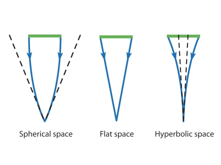
Flat universe from CMB • First peak: flat universe We know the redshift and the time it took for the light to reach us: from this we know the - length of the legs of the triangle - the angle at which we are measuring the sound horizon. Closed: hot spots appear larger Flat: appear as big as they are Open: spots appear smaller

The Cosmic Tonal Ladder The WMAP CMB temperature power spectrum Cosmic sound horizon The Cosmic Microwave Background Temperature Anisotropies: Universe is almost perfectly FLAT !!!!

Planck CMB Temperature Fluctuations

The WMAP CMB temperature power spectrum

FRW Universe: Curvature There is a 1 -1 relation between the total energy content of the Universe and its curvature. From FRW equations:

Cosmic Curvature & Cosmic Density SCP Union 2 constraints (2010) on values of matter density Ωm dark energy density ΩΛ