COSC 6335 Preprocessing Organization 1 2 3 Data

COSC 6335: Preprocessing Organization 1. 2. 3. Data Quality (already covered in part earlier) skip or Dec. 3 Data Preprocessing Methods (focus of this lecture) l Aggregation l Sampling l Dimensionality Reduction l Feature subset selection l Feature creation l Attribute Transformation l Discretization Similarity Assessment (already covered; part of the clustering transparencies) © Tan, Steinbach, Kumar edited by Ch. Eick Preprocessing in Data Mining 11/17/2020

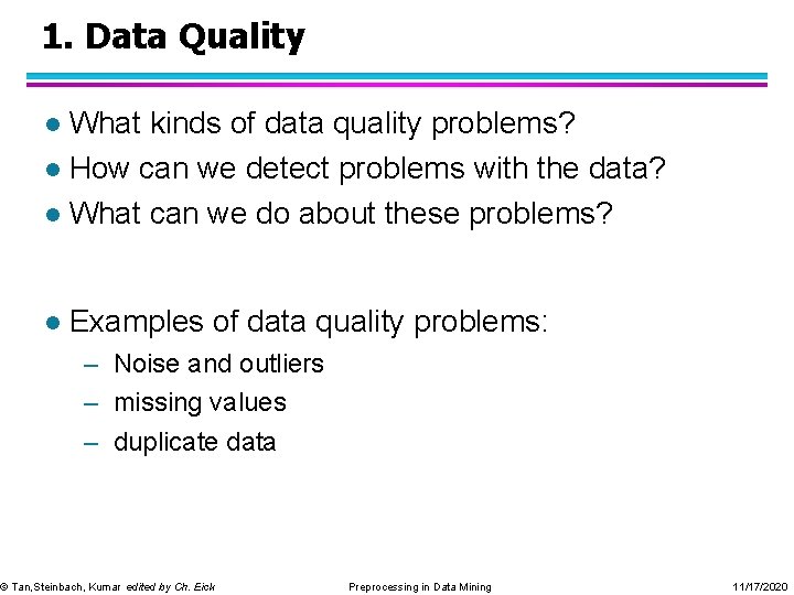
1. Data Quality What kinds of data quality problems? l How can we detect problems with the data? l What can we do about these problems? l l Examples of data quality problems: – Noise and outliers – missing values – duplicate data © Tan, Steinbach, Kumar edited by Ch. Eick Preprocessing in Data Mining 11/17/2020

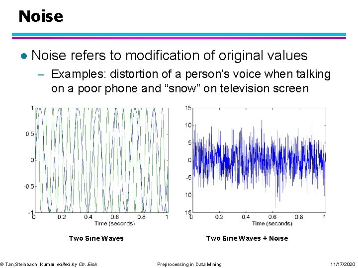
Noise l Noise refers to modification of original values – Examples: distortion of a person’s voice when talking on a poor phone and “snow” on television screen Two Sine Waves © Tan, Steinbach, Kumar edited by Ch. Eick Two Sine Waves + Noise Preprocessing in Data Mining 11/17/2020

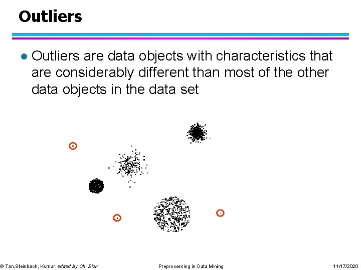
Outliers l Outliers are data objects with characteristics that are considerably different than most of the other data objects in the data set © Tan, Steinbach, Kumar edited by Ch. Eick Preprocessing in Data Mining 11/17/2020

Missing Values l Reasons for missing values – Information is not collected (e. g. , people decline to give their age and weight) – Attributes may not be applicable to all cases (e. g. , annual income is not applicable to children) l Handling missing values – – Eliminate Data Objects Estimate Missing Values Ignore the Missing Value During Analysis Replace with all possible values (weighted by their probabilities) – Learn a model that predicts the missing values © Tan, Steinbach, Kumar edited by Ch. Eick Preprocessing in Data Mining 11/17/2020

Duplicate Data l Data set may include data objects that are duplicates, or almost duplicates of one another – Major issue when merging data from heterogeous sources l Examples: – Same person with multiple email addresses – Duplicate Identifies in Medical Databases: http: //library. ahima. org/xpedio/groups/public/documents/ahima/bok 1_044000. hcsp? d. Doc. Name=bok 1_044000 l Data cleaning – Process of dealing with duplicate data issues © Tan, Steinbach, Kumar edited by Ch. Eick Preprocessing in Data Mining 11/17/2020

COSC 6335 News Dec. 1, 2020 A review list for the Dec 10, 2020, 2 p final exam will be available on the course website on the end of the day of Dec. 4. The final exam will take 115 minutes and counts 29% towards the overall grade. Ø For other news: see course webpage Ø Today: 1. Brief Introduction to Preprocessing 2. Group O’s Solution to the Silhouette Task 3. Brief Introduction to Spatial Data Mining (to be continued on Dec. 3) 4. 3: 15 p: Summary Kritik Poll and Kritik Discussion (all material can be found in the Kritik Poll DM 2020 channel) Ø © Tan, Steinbach, Kumar edited by Ch. Eick Preprocessing in Data Mining 11/17/2020

2. Data Preprocessing Methods Goal: Create a Data Set so that a Data Mining / Data Analysis method can be applied to it! Sub-activities of Data Preprocessing include: l Aggregation l Sampling l Dimensionality Reduction l Feature subset selection l Attribute Transformation l Feature creation l Discretization and Binning © Tan, Steinbach, Kumar edited by Ch. Eick Preprocessing in Data Mining 11/17/2020

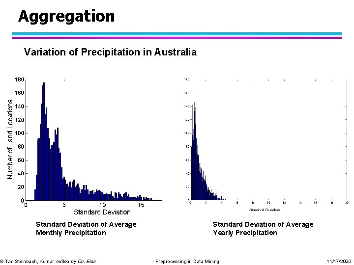
Aggregation Combining two or more attributes (or objects) into a single attribute (or object) l Purpose l – Data reduction u Reduce the number of attributes or objects – Change of scale u Cities aggregated into regions, states, countries, etc – More “stable” data u Aggregated data tends to have less variability © Tan, Steinbach, Kumar edited by Ch. Eick Preprocessing in Data Mining 11/17/2020

Aggregation Variation of Precipitation in Australia Standard Deviation of Average Monthly Precipitation © Tan, Steinbach, Kumar edited by Ch. Eick Standard Deviation of Average Yearly Precipitation Preprocessing in Data Mining 11/17/2020

Sampling l Sampling is the main technique employed for data selection. – It is often used for both the preliminary investigation of the data and the final data analysis. l Statisticians sample because obtaining the entire set of data of interest is too expensive or time consuming. l Sampling is used in data mining because processing the entire set of data of interest is too expensive or time consuming. © Tan, Steinbach, Kumar edited by Ch. Eick Preprocessing in Data Mining 11/17/2020

Sampling … l The key principle for effective sampling is the following: – using a sample will work almost as well as using the entire data sets, if the sample is representative – A sample is representative if it has approximately the same property (of interest) as the original set of data © Tan, Steinbach, Kumar edited by Ch. Eick Preprocessing in Data Mining 11/17/2020

Types of Sampling l Sampling without replacement – As each item is selected, it is removed from the population l Sampling with replacement – Objects are not removed from the population as they are selected for the sample. In sampling with replacement, the same object can be picked up more than once u l Stratified sampling – Split the data into several partitions; then draw random samples from each partition © Tan, Steinbach, Kumar edited by Ch. Eick Preprocessing in Data Mining 11/17/2020

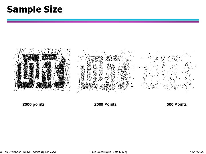
Sample Size 8000 points © Tan, Steinbach, Kumar edited by Ch. Eick 2000 Points Preprocessing in Data Mining 500 Points 11/17/2020

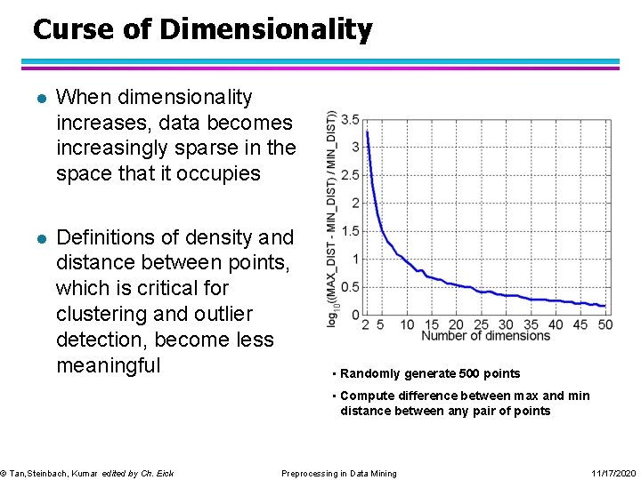
Curse of Dimensionality l When dimensionality increases, data becomes increasingly sparse in the space that it occupies l Definitions of density and distance between points, which is critical for clustering and outlier detection, become less meaningful © Tan, Steinbach, Kumar edited by Ch. Eick • Randomly generate 500 points • Compute difference between max and min distance between any pair of points Preprocessing in Data Mining 11/17/2020

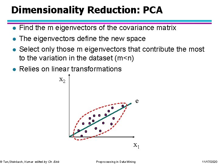
Dimensionality Reduction l Purpose: – Avoid curse of dimensionality – Reduce amount of time and memory required by data mining algorithms – Allow data to be more easily visualized – May help to eliminate irrelevant features or reduce noise l Techniques – – Principle Component Analysis Singular Value Decomposition Multi-dimensional Scaling … © Tan, Steinbach, Kumar edited by Ch. Eick Preprocessing in Data Mining 11/17/2020

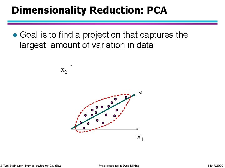
Dimensionality Reduction: PCA l Goal is to find a projection that captures the largest amount of variation in data x 2 © Tan, Steinbach, Kumar edited by Ch. Eick e x 1 Preprocessing in Data Mining 11/17/2020

Dimensionality Reduction: PCA l l Find the m eigenvectors of the covariance matrix The eigenvectors define the new space Select only those m eigenvectors that contribute the most to the variation in the dataset (m<n) Relies on linear transformations x 2 © Tan, Steinbach, Kumar edited by Ch. Eick e x 1 Preprocessing in Data Mining 11/17/2020

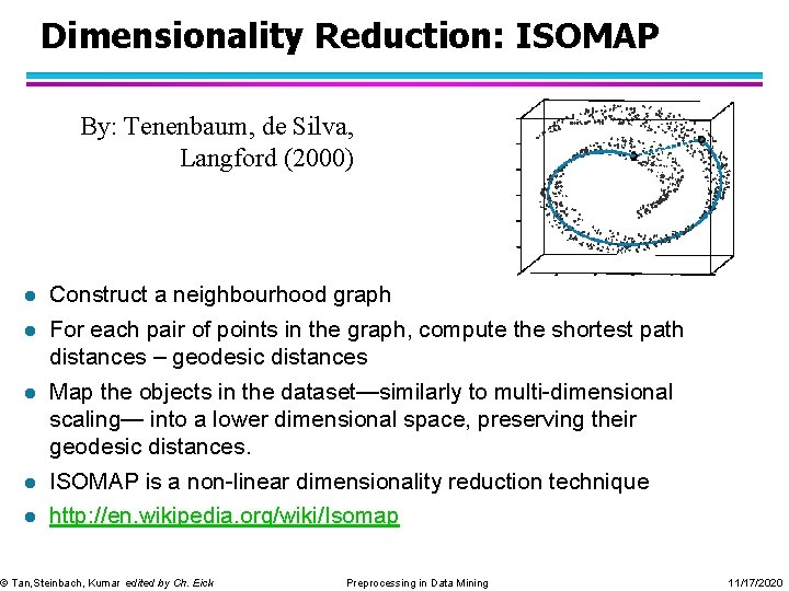
Dimensionality Reduction: ISOMAP By: Tenenbaum, de Silva, Langford (2000) l Construct a neighbourhood graph l For each pair of points in the graph, compute the shortest path distances – geodesic distances l Map the objects in the dataset—similarly to multi-dimensional scaling— into a lower dimensional space, preserving their geodesic distances. l ISOMAP is a non-linear dimensionality reduction technique l http: //en. wikipedia. org/wiki/Isomap © Tan, Steinbach, Kumar edited by Ch. Eick Preprocessing in Data Mining 11/17/2020

Feature Subset Selection Another way to reduce dimensionality of data l Redundant features l – duplicate much or all of the information contained in one or more other attributes – Example: purchase price of a product and the amount of sales tax paid l Irrelevant features – contain no information that is useful for the data mining task at hand – Example: students' ID is often irrelevant to the task of predicting students' GPA © Tan, Steinbach, Kumar edited by Ch. Eick Preprocessing in Data Mining 11/17/2020

Feature Subset Selection l skip or Dec. 3 Techniques: – Brute-force approch: u. Try all possible feature subsets as input to data mining algorithm – Embedded approaches: Feature selection occurs naturally as part of the data mining algorithm u – Filter approaches: u Features are selected before data mining algorithm is run – Wrapper approaches: Use the data mining algorithm as a black box to find best subset of attributes u © Tan, Steinbach, Kumar edited by Ch. Eick Preprocessing in Data Mining 11/17/2020

Feature Creation Create new attributes that can capture the important information in a data set much more efficiently than the original attributes. l Has gained a lot of popularity in the last 15 years through the introduction of kernels: http: //en. wikipedia. org/wiki/Kernel_method l General Idea: Either map data into a new space or augment dataset with newly created features. l © Tan, Steinbach, Kumar edited by Ch. Eick Preprocessing in Data Mining 11/17/2020

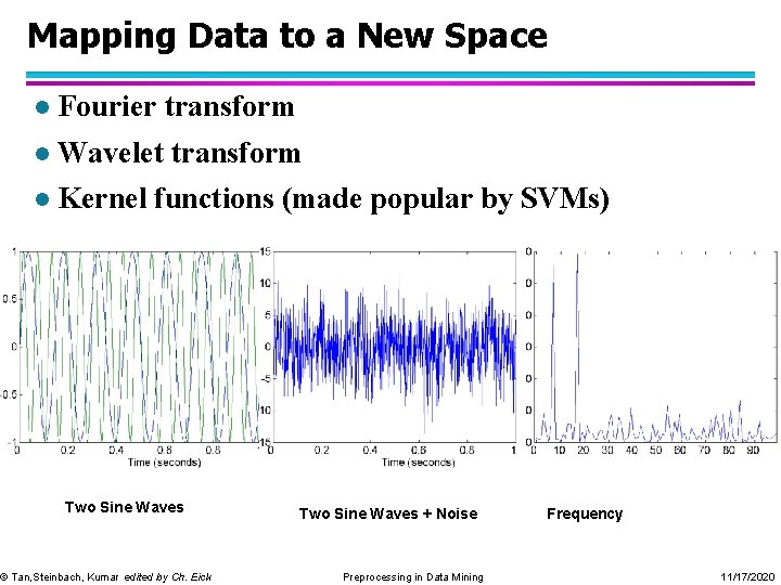
Mapping Data to a New Space l Fourier transform l Wavelet transform l Kernel functions (made popular by SVMs) Two Sine Waves © Tan, Steinbach, Kumar edited by Ch. Eick Two Sine Waves + Noise Preprocessing in Data Mining Frequency 11/17/2020

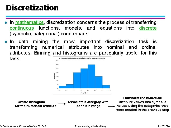
Discretization l In mathematics, discretization concerns the process of transferring continuous functions, models, and equations into discrete (symbolic, categorical) counterparts. l In data mining the most important discretization task is transforming numerical attributes into nominal and ordinal attributes. Binning and histograms are particularly useful for this task. Create histogram for the numerical attribute © Tan, Steinbach, Kumar edited by Ch. Eick Associate a category with each bin range Preprocessing in Data Mining Transform the numerical attribute values into symbolic values using the categories that were created in the previous step 11/17/2020

Similarity and Dissimilarity l Already covered! Similarity – Numerical measure of how alike two data objects are. – Is higher when objects are more alike. – Often falls in the range [0, 1] l Dissimilarity – Numerical measure of how different are two data objects – Lower when objects are more alike – Minimum dissimilarity is often 0 – Upper limit varies l Proximity refers to a similarity or dissimilarity © Tan, Steinbach, Kumar edited by Ch. Eick Preprocessing in Data Mining 11/17/2020

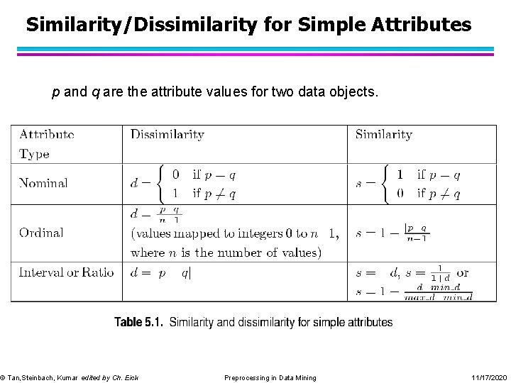
Similarity/Dissimilarity for Simple Attributes p and q are the attribute values for two data objects. © Tan, Steinbach, Kumar edited by Ch. Eick Preprocessing in Data Mining 11/17/2020

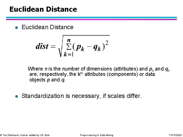
Euclidean Distance l Euclidean Distance Where n is the number of dimensions (attributes) and pk and qk are, respectively, the kth attributes (components) or data objects p and q. l Standardization is necessary, if scales differ. © Tan, Steinbach, Kumar edited by Ch. Eick Preprocessing in Data Mining 11/17/2020

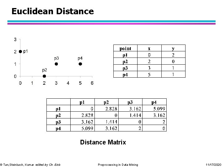
Euclidean Distance © Tan, Steinbach, Kumar edited by Ch. Eick Distance Matrix Preprocessing in Data Mining 11/17/2020

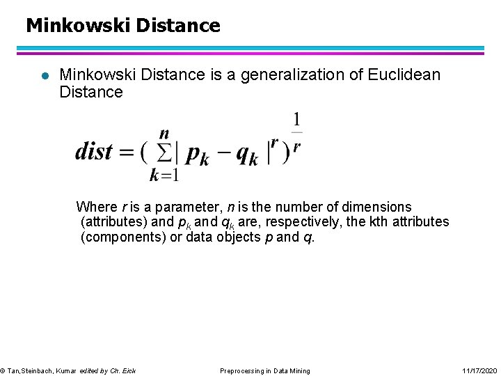
Minkowski Distance l Minkowski Distance is a generalization of Euclidean Distance Where r is a parameter, n is the number of dimensions (attributes) and pk and qk are, respectively, the kth attributes (components) or data objects p and q. © Tan, Steinbach, Kumar edited by Ch. Eick Preprocessing in Data Mining 11/17/2020

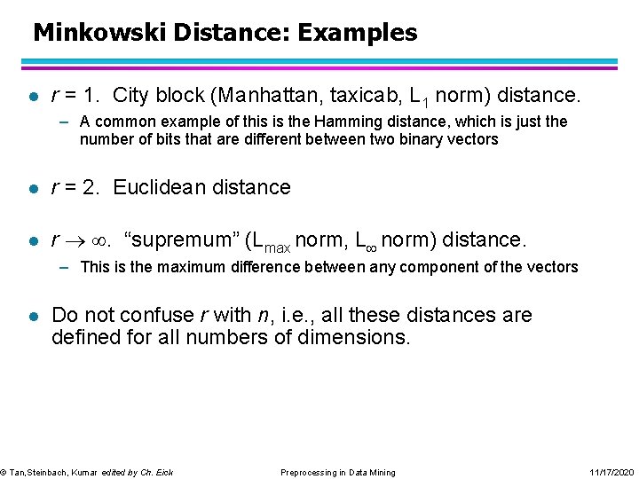
Minkowski Distance: Examples l r = 1. City block (Manhattan, taxicab, L 1 norm) distance. – A common example of this is the Hamming distance, which is just the number of bits that are different between two binary vectors l r = 2. Euclidean distance l r . “supremum” (Lmax norm, L norm) distance. – This is the maximum difference between any component of the vectors l Do not confuse r with n, i. e. , all these distances are defined for all numbers of dimensions. © Tan, Steinbach, Kumar edited by Ch. Eick Preprocessing in Data Mining 11/17/2020

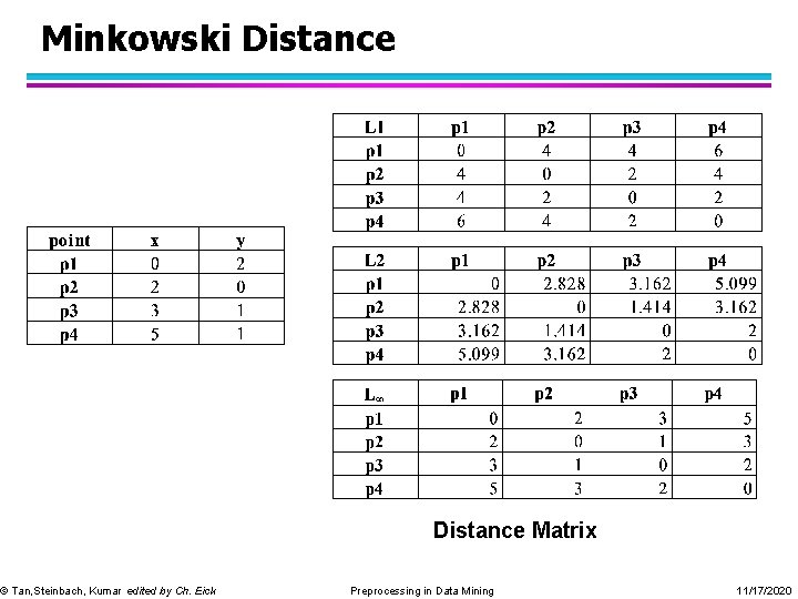
Minkowski Distance © Tan, Steinbach, Kumar edited by Ch. Eick Distance Matrix Preprocessing in Data Mining 11/17/2020

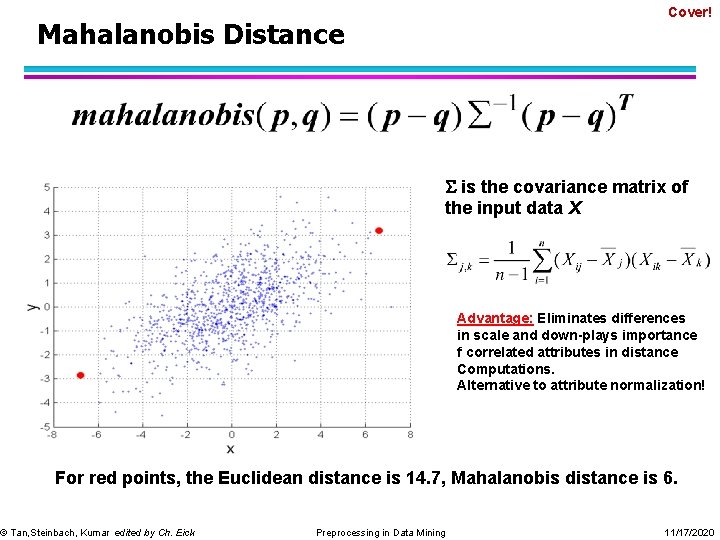
Cover! Mahalanobis Distance is the covariance matrix of the input data X Advantage: Eliminates differences in scale and down-plays importance f correlated attributes in distance Computations. Alternative to attribute normalization! For red points, the Euclidean distance is 14. 7, Mahalanobis distance is 6. © Tan, Steinbach, Kumar edited by Ch. Eick Preprocessing in Data Mining 11/17/2020

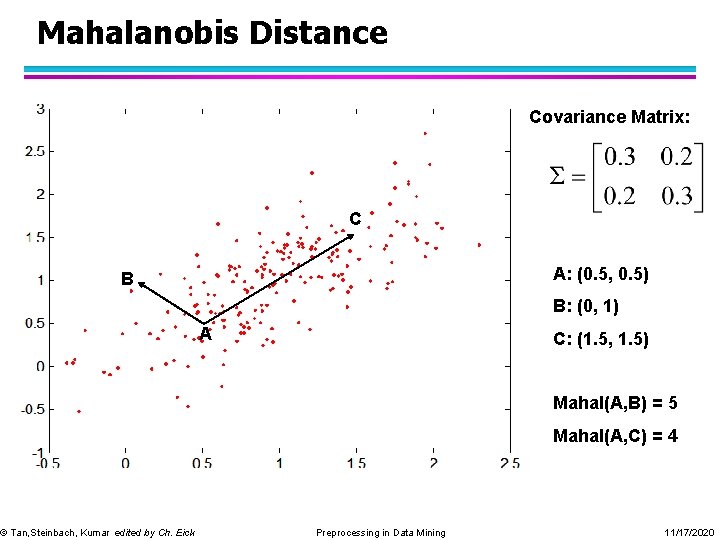
Mahalanobis Distance Covariance Matrix: C A: (0. 5, 0. 5) B © Tan, Steinbach, Kumar edited by Ch. Eick B: (0, 1) A C: (1. 5, 1. 5) Mahal(A, B) = 5 Mahal(A, C) = 4 Preprocessing in Data Mining 11/17/2020

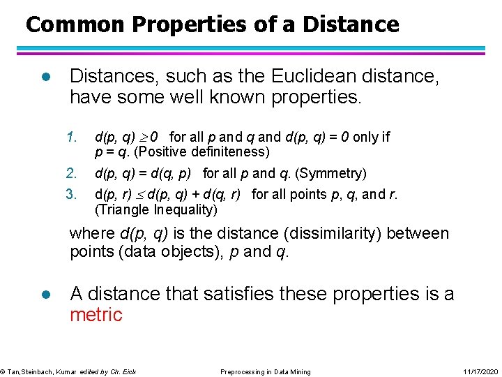
Common Properties of a Distance l Distances, such as the Euclidean distance, have some well known properties. 1. d(p, q) 0 for all p and q and d(p, q) = 0 only if p = q. (Positive definiteness) 2. 3. d(p, q) = d(q, p) for all p and q. (Symmetry) d(p, r) d(p, q) + d(q, r) for all points p, q, and r. (Triangle Inequality) where d(p, q) is the distance (dissimilarity) between points (data objects), p and q. l A distance that satisfies these properties is a metric © Tan, Steinbach, Kumar edited by Ch. Eick Preprocessing in Data Mining 11/17/2020

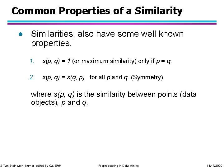
Common Properties of a Similarity l Similarities, also have some well known properties. 1. s(p, q) = 1 (or maximum similarity) only if p = q. 2. s(p, q) = s(q, p) for all p and q. (Symmetry) where s(p, q) is the similarity between points (data objects), p and q. © Tan, Steinbach, Kumar edited by Ch. Eick Preprocessing in Data Mining 11/17/2020

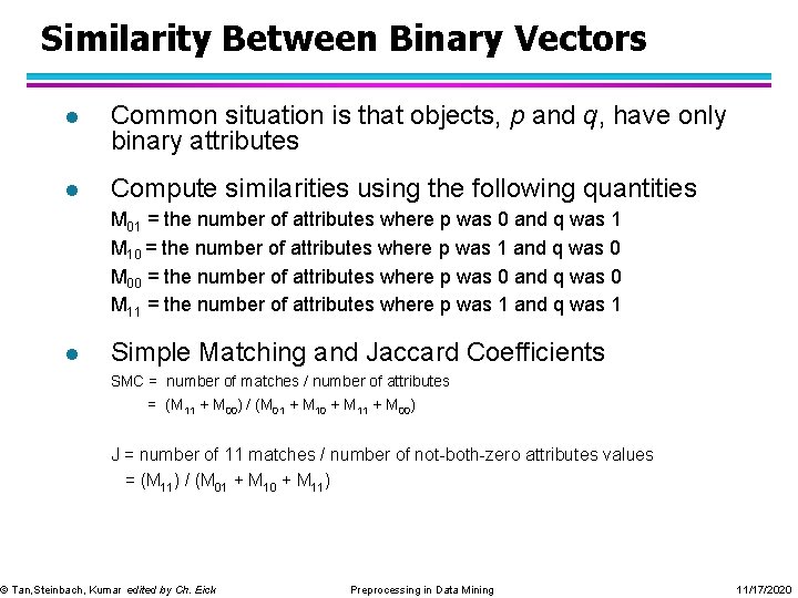
Similarity Between Binary Vectors l Common situation is that objects, p and q, have only binary attributes l Compute similarities using the following quantities M 01 = the number of attributes where p was 0 and q was 1 M 10 = the number of attributes where p was 1 and q was 0 M 00 = the number of attributes where p was 0 and q was 0 M 11 = the number of attributes where p was 1 and q was 1 l Simple Matching and Jaccard Coefficients SMC = number of matches / number of attributes = (M 11 + M 00) / (M 01 + M 10 + M 11 + M 00) J = number of 11 matches / number of not-both-zero attributes values = (M 11) / (M 01 + M 10 + M 11) © Tan, Steinbach, Kumar edited by Ch. Eick Preprocessing in Data Mining 11/17/2020

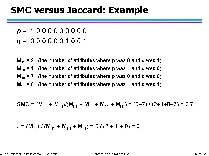
SMC versus Jaccard: Example p= 100000 q= 0000001001 M 01 = 2 (the number of attributes where p was 0 and q was 1) M 10 = 1 (the number of attributes where p was 1 and q was 0) M 00 = 7 (the number of attributes where p was 0 and q was 0) M 11 = 0 (the number of attributes where p was 1 and q was 1) SMC = (M 11 + M 00)/(M 01 + M 10 + M 11 + M 00) = (0+7) / (2+1+0+7) = 0. 7 J = (M 11) / (M 01 + M 10 + M 11) = 0 / (2 + 1 + 0) = 0 © Tan, Steinbach, Kumar edited by Ch. Eick Preprocessing in Data Mining 11/17/2020

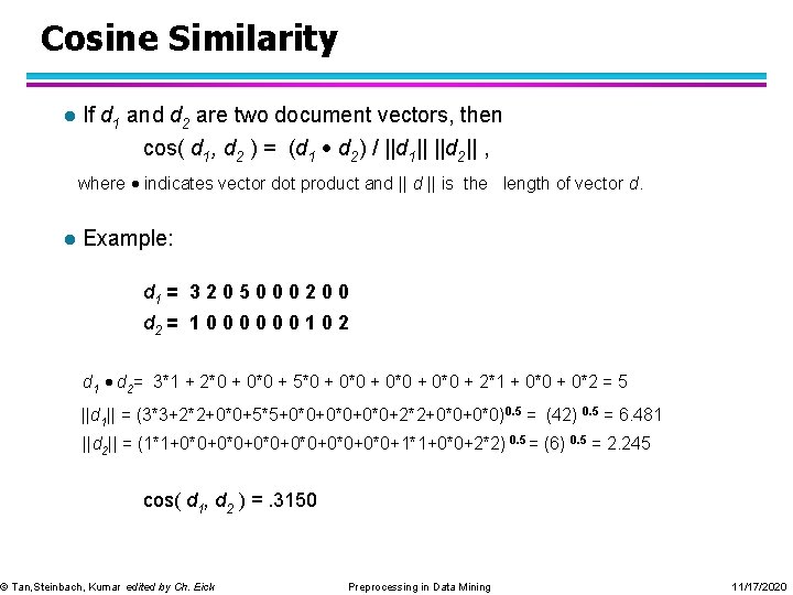
Cosine Similarity l If d 1 and d 2 are two document vectors, then cos( d 1, d 2 ) = (d 1 d 2) / ||d 1|| ||d 2|| , where indicates vector dot product and || is the length of vector d. l Example: d 1 = 3 2 0 5 0 0 0 2 0 0 d 2 = 1 0 0 0 1 0 2 d 1 d 2= 3*1 + 2*0 + 0*0 + 5*0 + 0*0 + 2*1 + 0*0 + 0*2 = 5 ||d 1|| = (3*3+2*2+0*0+5*5+0*0+0*0+2*2+0*0)0. 5 = (42) 0. 5 = 6. 481 ||d 2|| = (1*1+0*0+0*0+0*0+1*1+0*0+2*2) 0. 5 = (6) 0. 5 = 2. 245 cos( d 1, d 2 ) =. 3150 © Tan, Steinbach, Kumar edited by Ch. Eick Preprocessing in Data Mining 11/17/2020

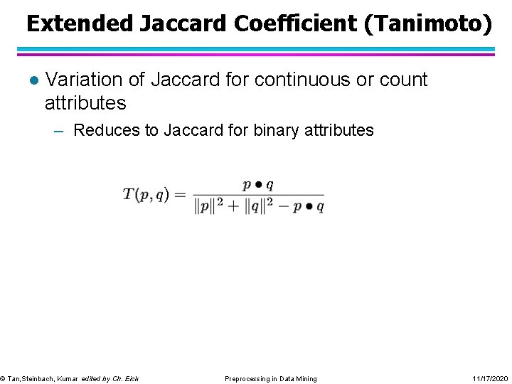
Extended Jaccard Coefficient (Tanimoto) l Variation of Jaccard for continuous or count attributes – Reduces to Jaccard for binary attributes © Tan, Steinbach, Kumar edited by Ch. Eick Preprocessing in Data Mining 11/17/2020

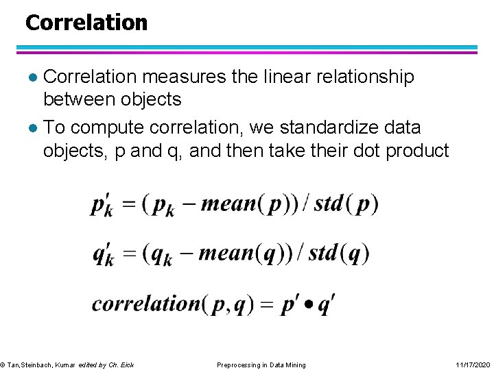
Correlation measures the linear relationship between objects l To compute correlation, we standardize data objects, p and q, and then take their dot product l © Tan, Steinbach, Kumar edited by Ch. Eick Preprocessing in Data Mining 11/17/2020

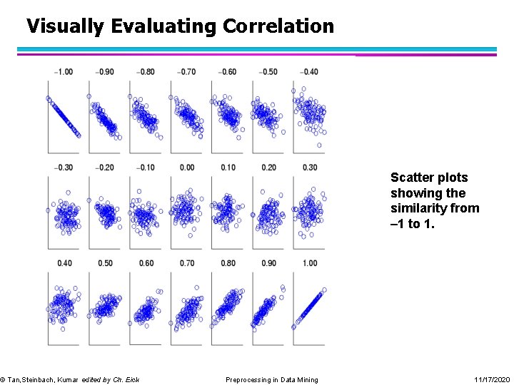
Visually Evaluating Correlation © Tan, Steinbach, Kumar edited by Ch. Eick Scatter plots showing the similarity from – 1 to 1. Preprocessing in Data Mining 11/17/2020