COSC 160 Data Structures Review Part 2 Jeremy

COSC 160: Data Structures Review – Part 2 Jeremy Bolton, Ph. D Assistant Teaching Professor

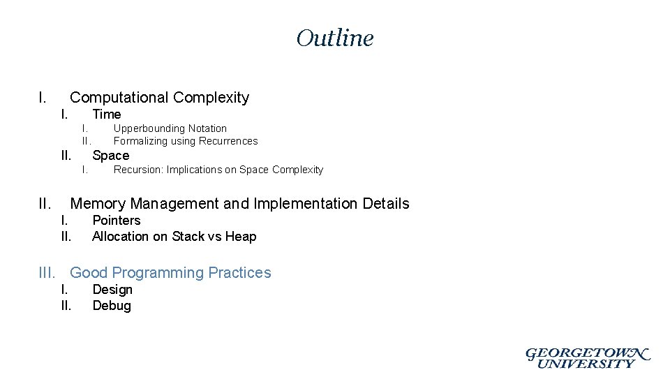
Outline I. Computational Complexity I. Time I. II. Space I. II. Upperbounding Notation Formalizing using Recurrences Recursion: Implications on Space Complexity Implementation Details I. II. Pointers Memory Management III. Good Programming Practices I. II. Design Debug

Review: Goals of Data Structures • Computer science is the practice of problem solving. – Data structures are tools used to help solve a problem or accomplish a task. – Good Solutions (Algorithms): • Good solutions are correct. • Good solutions are practical. • Good solutions are efficient. – Efficient in time – Efficient in space • Low level representations – Understanding lower level details related to memory management will make you a better programmer (of efficient structures and algorithms)

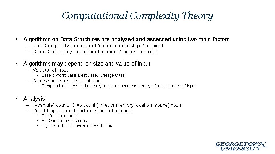
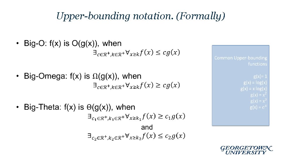
Computational Complexity Theory • Algorithms on Data Structures are analyzed and assessed using two main factors – Time Complexity – number of “computational steps” required. – Space Complexity – number of memory “spaces” required. • Algorithms may depend on size and value of input. – Value(s) of input • Cases: Worst Case, Best Case, Average Case. – Analysis in terms of size of input • Computational steps and memory requirements are generally a function of size of input. • Analysis – “Absolute” count: Step count (time) or memory location (space) count – Count Upper-bound and lower-bound notation: • Big-O: upper bound • Big-Omega: lower bound • Big-Theta: both upper and lower bound

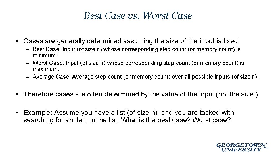
Best Case vs. Worst Case • Cases are generally determined assuming the size of the input is fixed. – Best Case: Input (of size n) whose corresponding step count (or memory count) is minimum. – Worst Case: Input (of size n) whose corresponding step count (or memory count) is maximum. – Average Case: Average step count (or memory count) over all possible inputs (of size n). • Therefore cases are often determined by the value of the input (not the size. ) • Example: Assume you have a list (of size n), and you are tasked with searching for an item in the list. What is the best case? Worst case?

Upper-bounding notation. (Formally) •

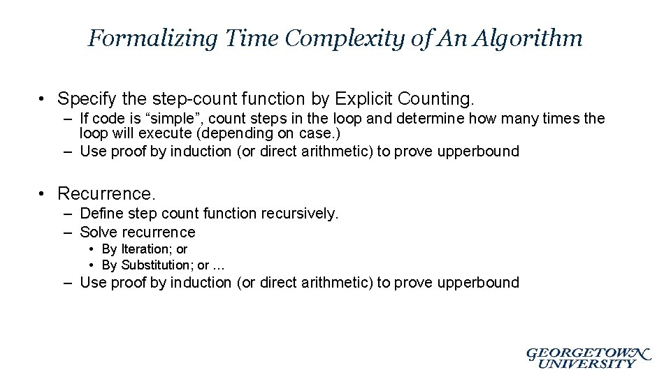
Formalizing Time Complexity of An Algorithm • Specify the step-count function by Explicit Counting. – If code is “simple”, count steps in the loop and determine how many times the loop will execute (depending on case. ) – Use proof by induction (or direct arithmetic) to prove upperbound • Recurrence. – Define step count function recursively. – Solve recurrence • By Iteration; or • By Substitution; or … – Use proof by induction (or direct arithmetic) to prove upperbound

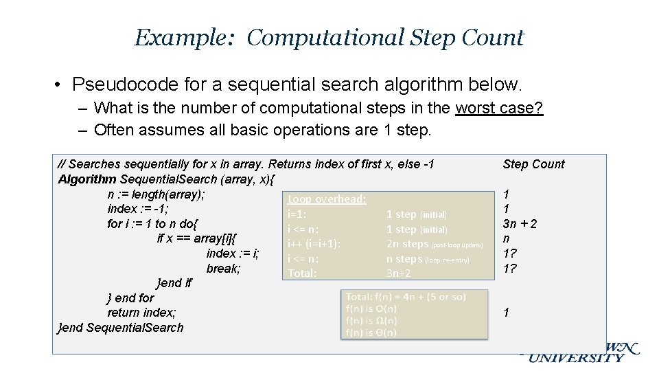
Example: Computational Step Count • Pseudocode for a sequential search algorithm below. – What is the number of computational steps in the worst case? – Often assumes all basic operations are 1 step. // Searches sequentially for x in array. Returns index of first x, else -1 Algorithm Sequential. Search (array, x){ n : = length(array); Loop overhead: index : = -1; i=1: 1 step (initial) for i : = 1 to n do{ i <= n: 1 step (initial) if x == array[i]{ i++ (i=i+1): 2 n steps (post-loop update) index : = i; i <= n: n steps (loop re-entry) break; Total: 3 n+2 }end if } end for return index; }end Sequential. Search Step Count 1 1 3 n + 2 n 1? 1? 1

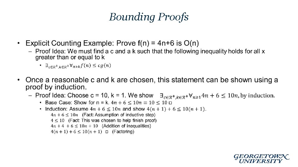
Bounding Proofs •

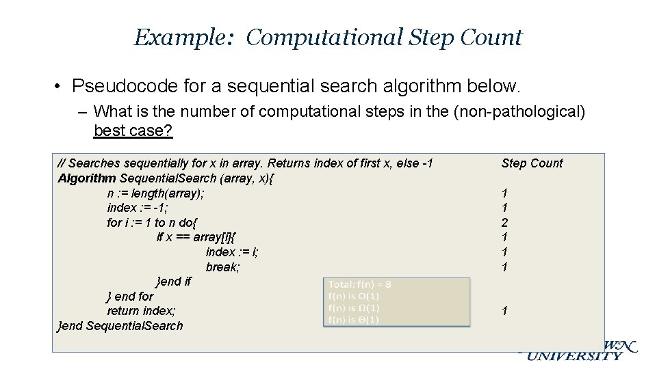
Example: Computational Step Count • Pseudocode for a sequential search algorithm below. – What is the number of computational steps in the (non-pathological) best case? // Searches sequentially for x in array. Returns index of first x, else -1 Algorithm Sequential. Search (array, x){ n : = length(array); index : = -1; for i : = 1 to n do{ if x == array[i]{ index : = i; break; }end if } end for return index; }end Sequential. Search Step Count 1 1 2 1 1

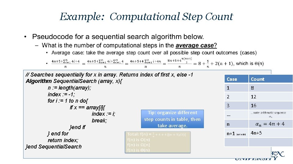
Example: Computational Step Count • // Searches sequentially for x in array. Returns index of first x, else -1 Algorithm Sequential. Search (array, x){ n : = length(array); index : = -1; for i : = 1 to n do{ if x == array[i]{ Tip: organize different index : = i; step counts in table, then break; take average. }end if } end for return index; }end Sequential. Search Case Count 1 8 2 12 3 16 … n n+1 (not in list) 4 n+5

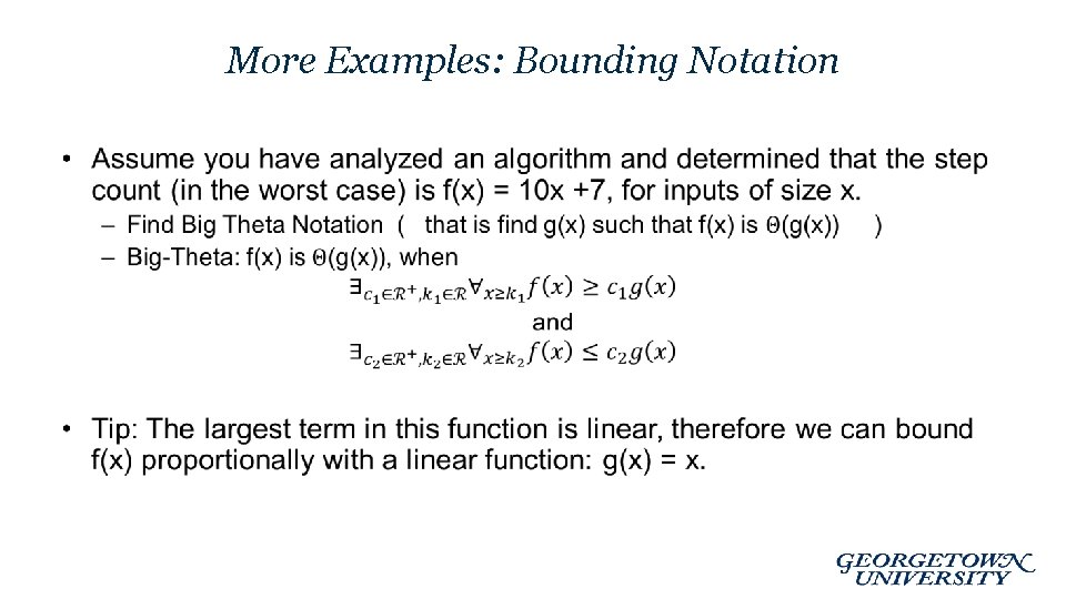
More Examples: Bounding Notation •

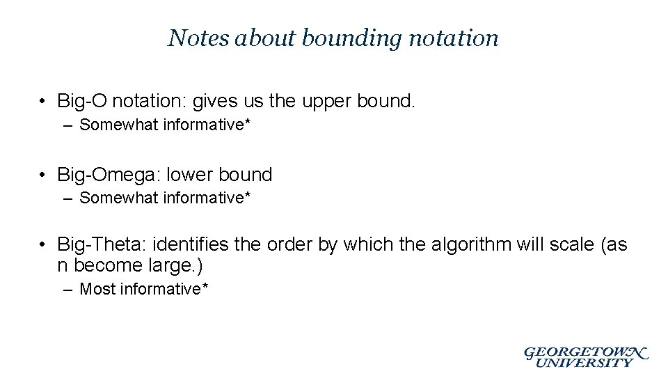
Notes about bounding notation • Big-O notation: gives us the upper bound. – Somewhat informative* • Big-Omega: lower bound – Somewhat informative* • Big-Theta: identifies the order by which the algorithm will scale (as n become large. ) – Most informative*

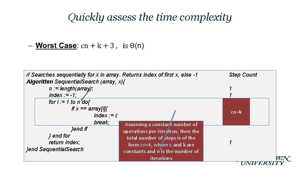
Quickly assess the time complexity • // Searches sequentially for x in array. Returns index of first x, else -1 Algorithm Sequential. Search (array, x){ n : = length(array); index : = -1; for i : = 1 to n do{ if x == array[i]{ index : = i; break; Assuming a constant number of }end if operations per iteration, then the } end for total number of steps is of the return index; form cn+k, where c and k are }end Sequential. Search constants and n is the number of iterations Step Count 1 1 3 n + 2 n cn+k 1 1 1

Time Complexity using Recurrences • Recursion – Defining an entity in terms of itself • Recurrence – A relation that characterizes a function in terms of its value on a smaller input • General Idea: – Many computer science solutions can be defined recursively – Similarly, many step count functions can be defined using a recurrence

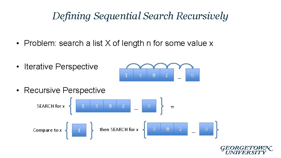
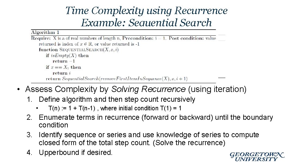
Defining Sequential Search Recursively • Problem: search a list X of length n for some value x • Iterative Perspective 1 3 8 2 … 0 2 … • Recursive Perspective SEARCH for x Compare to x 1 1 3 8 2 … then SEARCH for x = 0 3 8 0

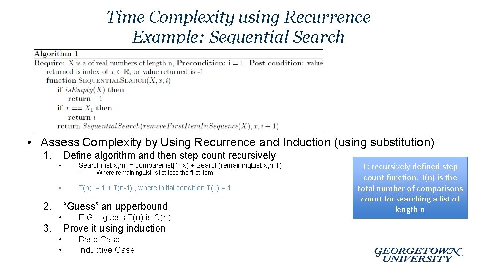
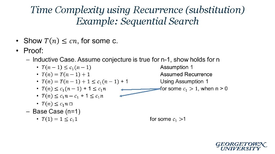
Time Complexity using Recurrence Example: Sequential Search • Assess Complexity by Using Recurrence and Induction (using substitution) 1. Define algorithm and then step count recursively • Search(list, x, n) : = compare(list[1], x) + Search(remaining. List, x, n-1) – • 2. Where remaining. List is list less the first item T(n) : = 1 + T(n-1) , where initial condition T(1) = 1 “Guess” an upperbound • 3. E. G. I guess T(n) is O(n) Prove it using induction • • Base Case Inductive Case T: recursively defined step count function. T(n) is the total number of comparisons count for searching a list of length n

Time Complexity using Recurrence (substitution) Example: Sequential Search •

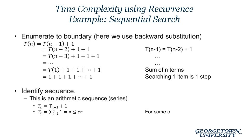
Time Complexity using Recurrence Example: Sequential Search • Assess Complexity by Solving Recurrence (using iteration) 1. Define algorithm and then step count recursively • T(n) : = 1 + T(n-1) , where initial condition T(1) = 1 2. Enumerate terms in recurrence (forward or backward) until the boundary condition 3. Identify sequence or series and use knowledge of series to compute closed form of the total step count. (Solve the recurrence) 4. Upperbound if desired.

Time Complexity using Recurrence Example: Sequential Search •

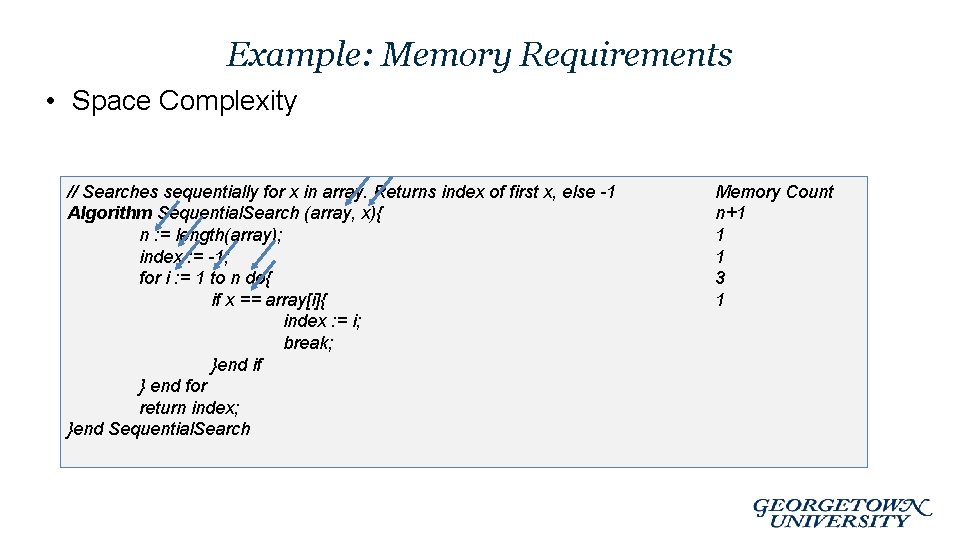
Example: Memory Requirements • Space Complexity // Searches sequentially for x in array. Returns index of first x, else -1 Algorithm Sequential. Search (array, x){ n : = length(array); index : = -1; for i : = 1 to n do{ if x == array[i]{ index : = i; break; }end if } end for return index; }end Sequential. Search Memory Count n+1 1 1 3 1

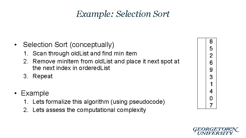
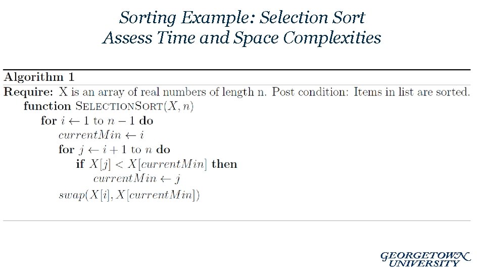
Example: Selection Sort • Selection Sort (conceptually) 1. Scan through old. List and find min item 2. Remove min. Item from old. List and place it next spot at the next index in ordered. List 3. Repeat • Example 1. Lets formalize this algorithm (using pseudocode) 2. Lets assess the computational complexity

Recall: Definition of an Algorithm • PROPERTIES OF ALGORITHMS – Input domain is defined – Output domain is specified – The output or result is correct • Preconditions: logical statements assumed to be true prior to algorithm execution • Postconditions: logical statements assumed to be true after algorithm execution – The constituent steps are well-defined – Each step is performable in finite time

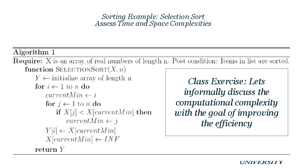
Sorting Example: Selection Sort Assess Time and Space Complexities Class Exercise: Lets informally discuss the computational complexity with the goal of improving the efficiency

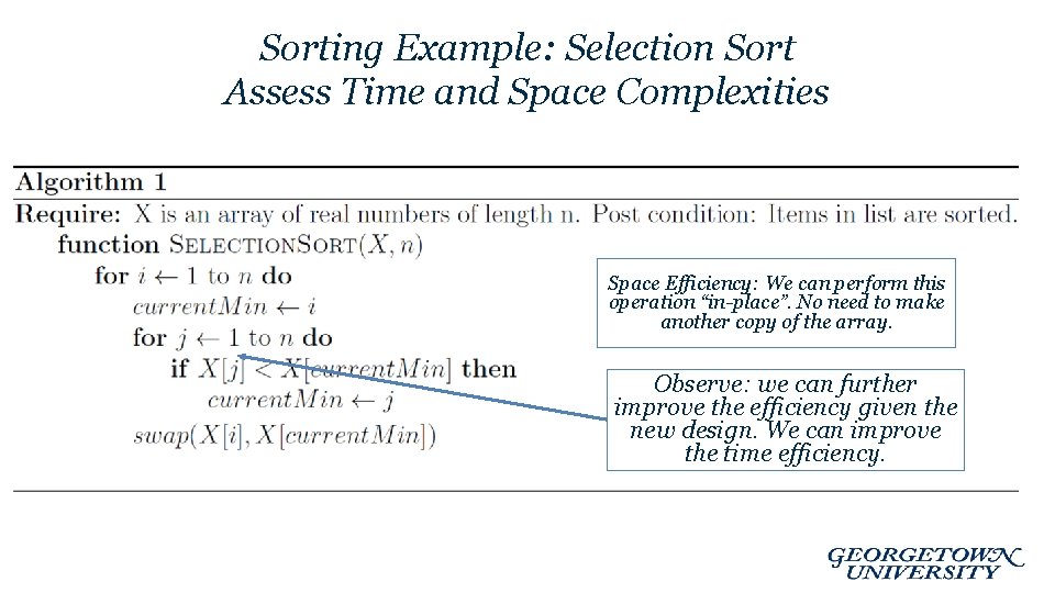
Sorting Example: Selection Sort Assess Time and Space Complexities Space Efficiency: We can perform this operation “in-place”. No need to make another copy of the array. Observe: we can further improve the efficiency given the new design. We can improve the time efficiency.

Sorting Example: Selection Sort Assess Time and Space Complexities

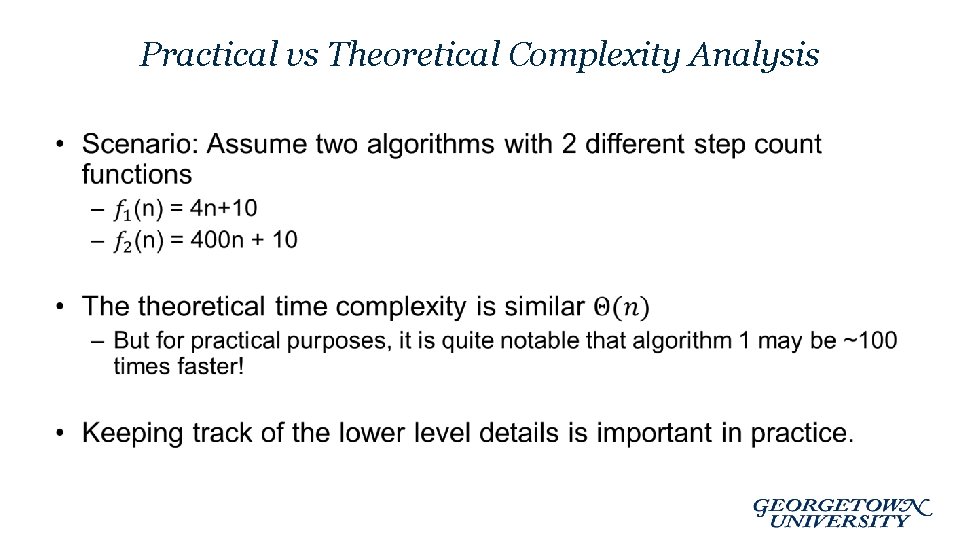
Practical vs Theoretical Complexity Analysis •

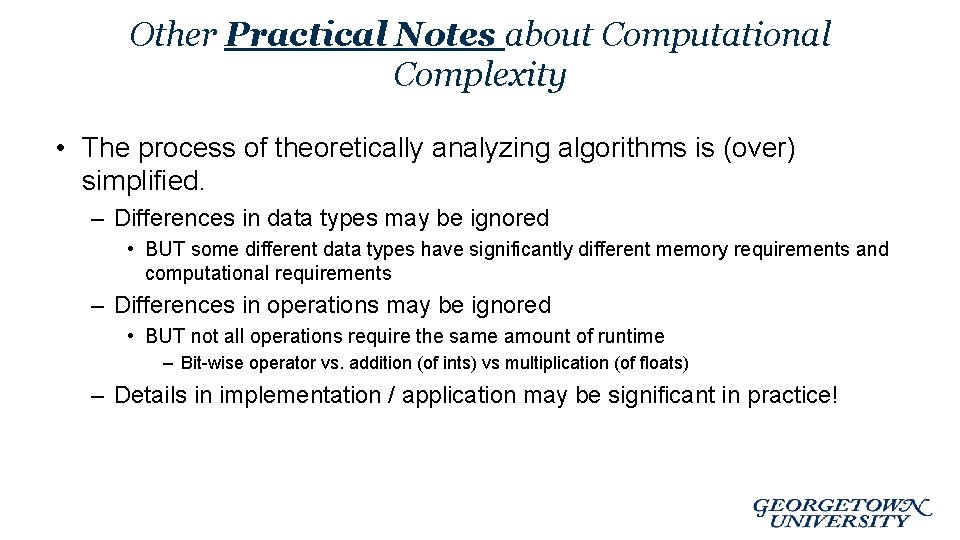
Other Practical Notes about Computational Complexity • The process of theoretically analyzing algorithms is (over) simplified. – Differences in data types may be ignored • BUT some different data types have significantly different memory requirements and computational requirements – Differences in operations may be ignored • BUT not all operations require the same amount of runtime – Bit-wise operator vs. addition (of ints) vs multiplication (of floats) – Details in implementation / application may be significant in practice!

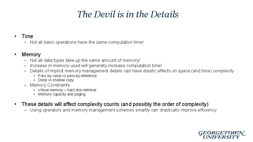
The Devil is in the Details • Time – Not all basic operations have the same computation time! • Memory – Not all data types take up the same amount of memory! – Increase in memory used will generally increase computation time! – Details of implicit memory management details can have drastic effects on space (and time) complexity • Pass by value vs pass-by-reference • Deep vs shallow copy – Memory Constraints • Virtual memory – hard disk retrieval • Memory capacity and paging • These details will affect complexity counts (and possibly the order of complexity) – Using operators and memory management schemes smartly can drastically improve efficiency

Outline I. Computational Complexity I. Time I. II. Space I. II. Upperbounding Notation Formalizing using Recurrences Recursion: Implications on Space Complexity Memory Management and Implementation Details I. II. Pointers Allocation on Stack vs Heap III. Good Programming Practices I. II. Design Debug

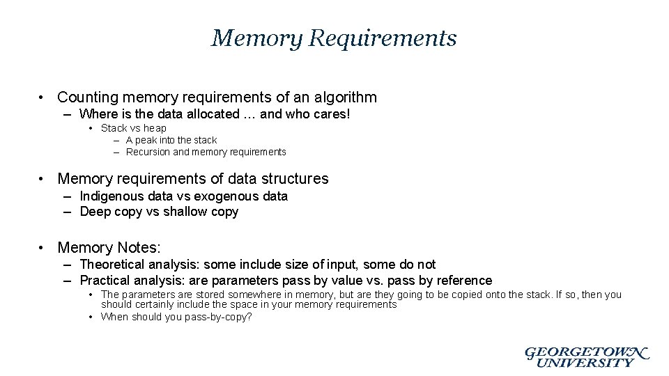
Memory Requirements • Counting memory requirements of an algorithm – Where is the data allocated … and who cares! • Stack vs heap – A peak into the stack – Recursion and memory requirements • Memory requirements of data structures – Indigenous data vs exogenous data – Deep copy vs shallow copy • Memory Notes: – Theoretical analysis: some include size of input, some do not – Practical analysis: are parameters pass by value vs. pass by reference • The parameters are stored somewhere in memory, but are they going to be copied onto the stack. If so, then you should certainly include the space in your memory requirements • When should you pass-by-copy?

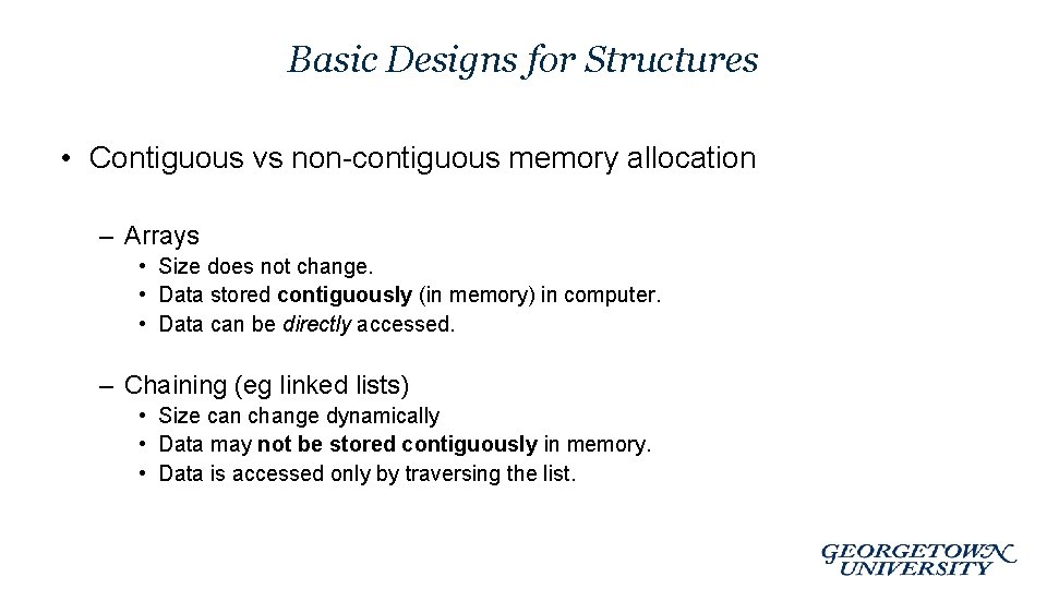
Basic Designs for Structures • Contiguous vs non-contiguous memory allocation – Arrays • Size does not change. • Data stored contiguously (in memory) in computer. • Data can be directly accessed. – Chaining (eg linked lists) • Size can change dynamically • Data may not be stored contiguously in memory. • Data is accessed only by traversing the list.

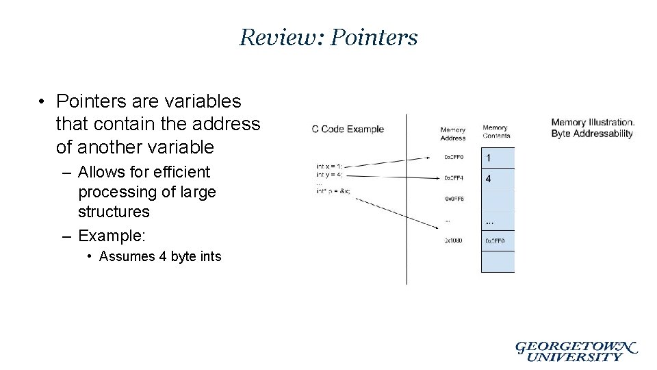
Review: Pointers • Pointers are variables that contain the address of another variable – Allows for efficient processing of large structures – Example: • Assumes 4 byte ints

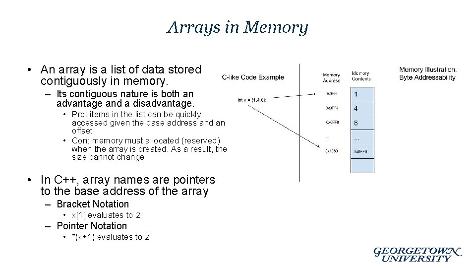
Arrays in Memory • An array is a list of data stored contiguously in memory. – Its contiguous nature is both an advantage and a disadvantage. • Pro: items in the list can be quickly accessed given the base address and an offset • Con: memory must allocated (reserved) when the array is created. As a result, the size cannot change. • In C++, array names are pointers to the base address of the array – Bracket Notation • x[1] evaluates to 2 – Pointer Notation • *(x+1) evaluates to 2

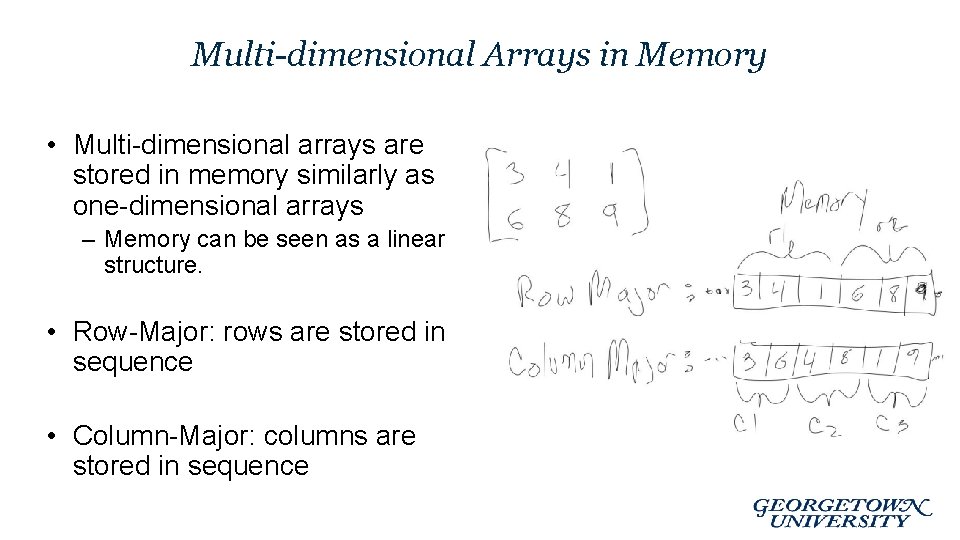
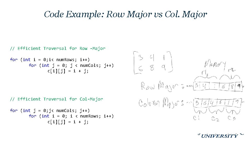
Multi-dimensional Arrays in Memory • Multi-dimensional arrays are stored in memory similarly as one-dimensional arrays – Memory can be seen as a linear structure. • Row-Major: rows are stored in sequence • Column-Major: columns are stored in sequence

Lists using “Chaining” • Some lists can change size once created. This is generally accomplished by chaining. – The data cannot necessarily be stored contiguously in memory in this instance (as the memory is not allocated at one time. ) Thus the data may not be sequentially contiguous in memory. • But then how can we access items in the list? • This extra flexibility comes at the cost of storing 1 pointer per data item stored. This pointer will point to the next item in the list, thus facilitating a “linked” list. • A linked (or chained) structure in memory

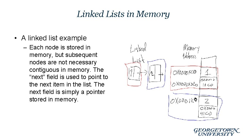
Linked Lists in Memory • A linked list example – Each node is stored in memory, but subsequent nodes are not necessary contiguous in memory. The “next” field is used to point to the next item in the list. The next field is simply a pointer stored in memory.

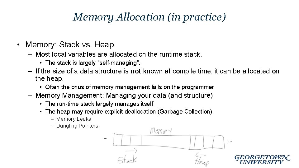
Memory Allocation (in practice) • Memory: Stack vs. Heap – Most local variables are allocated on the runtime stack. • The stack is largely “self-managing”. – If the size of a data structure is not known at compile time, it can be allocated on the heap. • Often the onus of memory management falls on the programmer – Memory Management: Managing your data (and structure) • The run-time stack largely manages itself • The heap may require explicit deallocation (Garbage Collection). – Memory Leaks. – Dangling Pointers … …

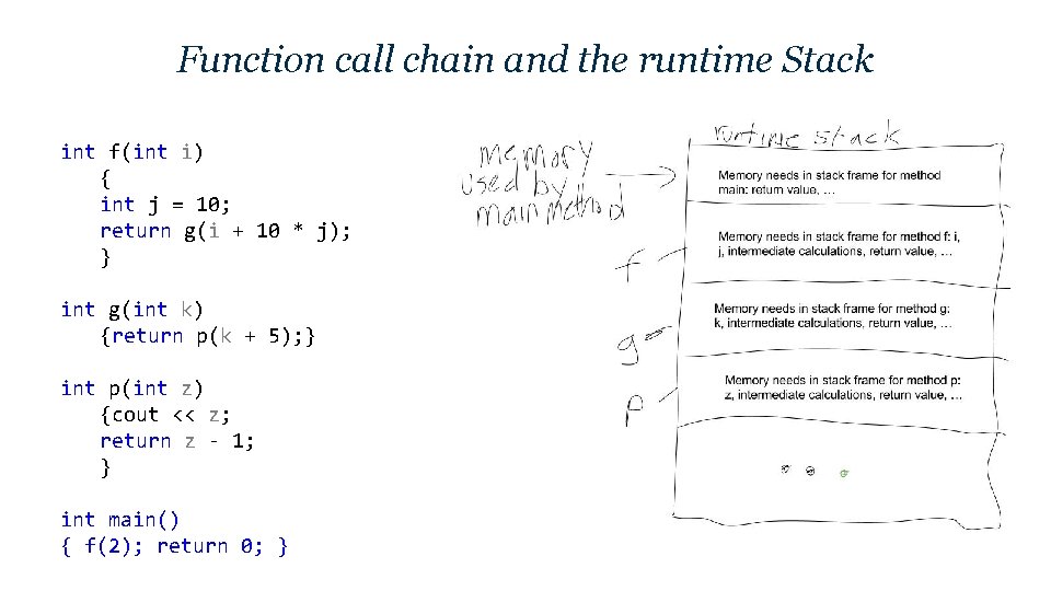
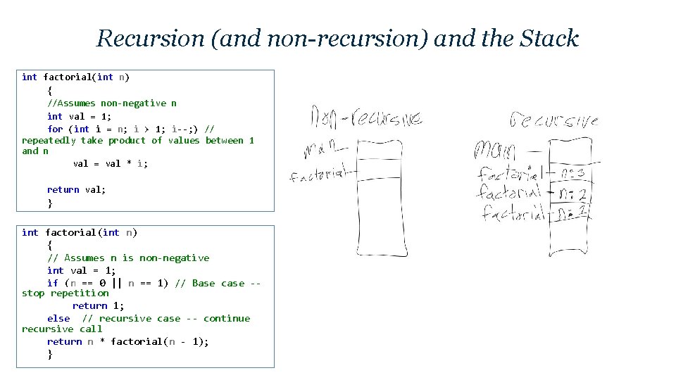
Memory and the Runtime Stack (in practice) • In most programming languages, when a new scope is opened, (e. g. a function is called), a new frame of memory is reserved for all variables local to that scope (as well as some memory other data / variables such as input parameters, return values, intermediate calculations, … ). • Each scope or frame of memory is reserved on a dynamicallyallocated, contiguous portion of memory referred to as the runtime stack. – Function call chains – Recursion example

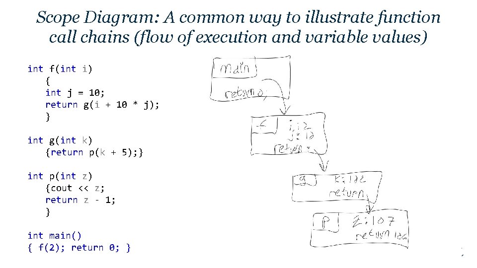
Scope Diagram: A common way to illustrate function call chains (flow of execution and variable values) int f(int i) { int j = 10; return g(i + 10 * j); } int g(int k) {return p(k + 5); } int p(int z) {cout << z; return z - 1; } int main() { f(2); return 0; }

Function call chain and the runtime Stack int f(int i) { int j = 10; return g(i + 10 * j); } int g(int k) {return p(k + 5); } int p(int z) {cout << z; return z - 1; } int main() { f(2); return 0; }

Recursion • Recursive methods can greatly impact memory allocation • Recursive methods are methods that are defined in terms of themselves. • Many processes and calculations that involve repetition can be implemented recursively.

Recursion Example: Factorial • Write a function to calculate n! where n is the input argument n! = n*(n-1)*(n-2)*… *2*1 n! = n*(n-1)! factorial(n) =n*factorial(n-1) • Note that this calculation is inherently repetitive. – There is repeated multiplication to be performed – Further note that the number of multiplications is dependent on “n” that is the input parameter will control the number of repetitive computations (multiplications in this case)

Factorial Examples int factorial(int n) { //Assumes non-negative n int val = 1; for (int i = n; i > 1; i--; ) // repeatedly take product of values between 1 and n val = val * i; return val; } int factorial(int n) { // Assumes n is non-negative int val = 1; if (n == 0 || n == 1) // Base case -stop repetition return 1; else // recursive case -- continue recursive call return n * factorial(n - 1); }

Draw Scope (function chain) diagrams to trace the execution of a recursive function. int f(int n) { // Assumes n is non-negative int val = 1; if (n == 0 || n == 1) // Base case -- stop repetition return 1; else // recursive case -- continue recursive call return n * f(n - 1); } void main() {f(3); }

Recursion (and non-recursion) and the Stack int factorial(int n) { //Assumes non-negative n int val = 1; for (int i = n; i > 1; i--; ) // repeatedly take product of values between 1 and n val = val * i; return val; } int factorial(int n) { // Assumes n is non-negative int val = 1; if (n == 0 || n == 1) // Base case -stop repetition return 1; else // recursive case -- continue recursive call return n * factorial(n - 1); }

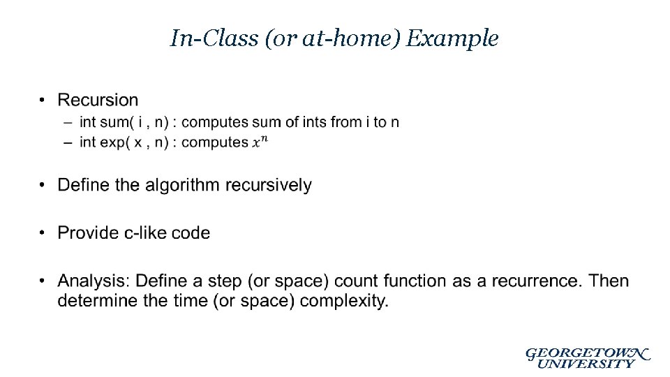
In-Class (or at-home) Example •

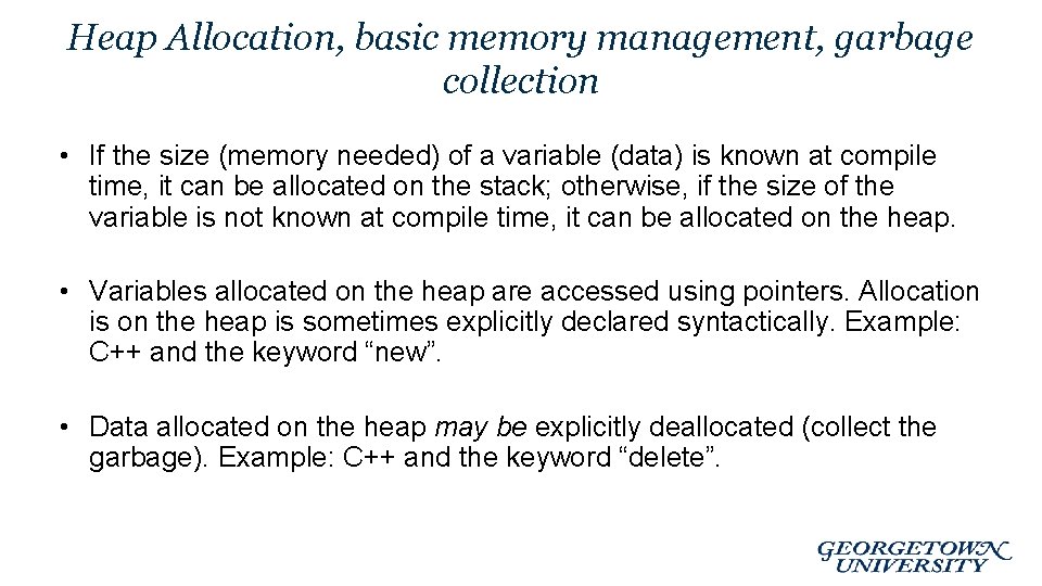
Heap Allocation, basic memory management, garbage collection • If the size (memory needed) of a variable (data) is known at compile time, it can be allocated on the stack; otherwise, if the size of the variable is not known at compile time, it can be allocated on the heap. • Variables allocated on the heap are accessed using pointers. Allocation is on the heap is sometimes explicitly declared syntactically. Example: C++ and the keyword “new”. • Data allocated on the heap may be explicitly deallocated (collect the garbage). Example: C++ and the keyword “delete”.

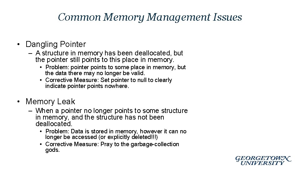
Common Memory Management Issues • Dangling Pointer – A structure in memory has been deallocated, but the pointer still points to this place in memory. • Problem: pointer points to some place in memory, but the data there may no longer be valid. • Corrective Measure: Set pointer to null to clearly indicate pointer points nowhere. • Memory Leak – When a pointer no longer points to some structure in memory, and the structure has not been deallocated. • Problem: Data is stored in memory, however it can no longer be accessed (or explicitly deleted!!!) • Corrective Measure: Pray to the garbage-collection gods.

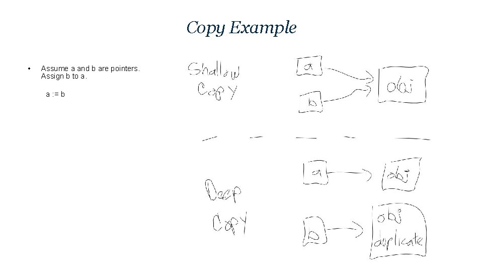
Memory Usage (cont): Deep vs Shallow Copy • Data is copied often in computer programs – Assignment – Parameter passing – Return values • Shallow copy – a simple bitwise copy. – May (or may not) be good when dealing with pointers – EG: pass by reference • Deep copy – pointers are dereferenced and the data pointed to by the pointer is copied. – EG (C++): overloading the =operator or copy constructor

Copy Example • Assume a and b are pointers. Assign b to a. a : = b

Data Storage Hierarchy (in practice) • Another practical issue related to algorithm analysis and implementation is RAM limitations and retrieving data from secondary storage. – Over-Simplified Summary: Retrieving data from secondary storage is very slow, and thus data is loaded to cache and RAM memory for processing. RAM is very versatile but has limitations. Some data structures may be large enough such that data will need to be continuously retrieved and restored back to secondary storage (thrashing). – Understanding RAM and Caching limitations and schemes on a computer is important when designing large data structures. • Possible ways to mitigate these issues – Localize processing to subsets of the data. – Traverse and organize data smartly • Row-major vs column major

Code Example: Row Major vs Col. Major // Efficient Traversal for Row -Major for (int i = 0; i< num. Rows; i++) for (int j = 0; j < num. Cols; j++) c[i][j] = i + j; // Efficient Traversal for Col-Major for (int j = 0; j< num. Cols; j++) for (int i = 0; i < num. Rows; i++) c[i][j] = i + j;

Outline I. Computational Complexity I. Time I. II. Space I. II. Upperbounding Notation Formalizing using Recurrences Recursion: Implications on Space Complexity Memory Management and Implementation Details I. II. Pointers Allocation on Stack vs Heap III. Good Programming Practices I. II. Design Debug

Good Structure Design Schemes • Project design details are largely up to you, but I encourage you to abide by good coding practices. – This will benefit you and anyone who might use or read your code. • Design for usability, reusability, efficiency, …. – Object Oriented Programming Design • Inheritance (writeability, reusability ) • Encapsulation (reliability) • (Poly) Dynamic dispatch (writeability, flexibility, reusability) – Templates • Explicit “polymorphism” (reusability, writeability) • Some simple computational complexity tips

OOP Design • Classes / Structs provide for a fitting programming construct to represent data structures. • Appropriately designing classes and class hierarchies will improve the effectiveness of your code – Reusability – Readability – Writeablility

Templates in C++ • Templates / Generics allow for explicit “polymorphism” which promotes – – Flexibility Reusability Readability Writeablility

Debugging and Testing • Time distribution: – Planning Designing: 1/3 – Actual Coding: 1/3 – Testing / Debugging: 1/3 • Design a good testing scheme for your software. – Repeatedly code, then test, … – In theory, you want to assure that your program produces the correct output for all possible inputs – In practice, select a subset of inputs that “efficiently” test your program. • EG: Include test input values such that each branch in execution flow is tested.

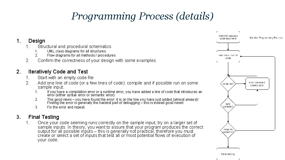
Programming Process (details) 1. Design 1. Structural and procedural schematics 1. 2. 2. Confirm the correctness of your design with some examples. Iteratively Code and Test 1. 2. Start with an empty code file Add one line of code (or a few lines of code): compile and if possible run on some sample input. 1. 2. 3. UML class diagrams for all structures. Flow diagrams for all methods / procedures If you have a compilation error or a runtime error, you have added a line of code that introduces an error (either syntax error or semantic error). The good news – you have found the error: it is on the line you have just added (almost always)! Finding the error is generally the hardest part of debugging – this is indeed good news! Fix the error and repeat. Final Testing 1. Once your code seeming runs correctly on the sample input, try on a larger set of sample inputs. In theory, you want to assure that your program produces the correct output for all possible inputs – this is generally not practical, therefore you must create or select a set of inputs that test all or most potential flows of execution of your code.

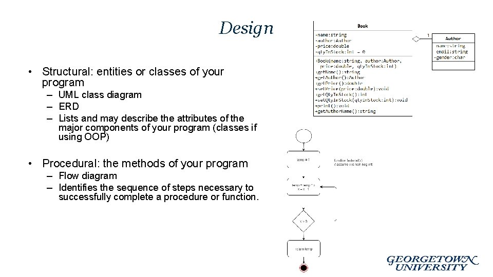
Design • Structural: entities or classes of your program – UML class diagram – ERD – Lists and may describe the attributes of the major components of your program (classes if using OOP) • Procedural: the methods of your program – Flow diagram – Identifies the sequence of steps necessary to successfully complete a procedure or function.

Some Final Computational Complexity Tips • Time – – – If possible, remove statements from loops. If possible, use operators that are fast. Avoid excessive recursion. Use mathematical properties to your advantage Use practical understanding of computers to your advantage. • Memory – Large structures: • Pass by reference / global* • Manage large structures “intelligently” to account for memory / hardware delays – Use “minimally sufficient” data types • EG: Don’t use a double if an int will suffice. – Avoid (excessive) recursion (unnecessary memory usage). – Use practical understanding of computers to your advantage.