Correlational NonExperimental Design Presenters Dr Armando Paladino 1

Correlational Non-Experimental Design Presenters: Dr. Armando Paladino 1

2 Correlational Designs: Relational & Predictive

3 Presentation Outline When To Use Types Characteristics Assumptions Mediation

4 Correlational Designs When do we use the design? This design is appropriate for exploring problems about the relationships between constructs, construct dimensions and items on a scale. For example, the age of a child may be related to the height and the adult occupation may be related to his/her income level (Cohen, West, & Aiken, 2003) Types Relational This design is used to identify the existence, strength and direction of relationships between two variables. The synonym of correlation is “association”, and it is referred to the direction and magnitude of the relationship between two variables. The supporting analysis is correlation. Predictive This design is used to identify predictive relationships between the predictor(s) and the outcome(s)/criterion variable(s). The supporting analysis is the regression analysis (different types).

5 Correlational Designs The Pearson product-moment correlation is used to determine the strength and direction of a linear relationship between two continuous variables. More specifically, the test generates a coefficient called the Pearson correlation coefficient, denoted as r (i. e. , the italic lowercase letter r), and it is this coefficient that measures the strength and direction of a linear relationship between two continuous variables. Its value can range from -1 for a perfect negative linear relationship to +1 for a perfect positive linear relationship. A value of 0 (zero) indicates no relationship between two variables. This test is also known by its shorter titles, the Pearson correlation or Pearson's correlation, which are often used interchangeably. You could use multiple regression to understand whether exam performance can be predicted based on revision time, test anxiety, lecture attendance, course studied and gender. Here, your continuous dependent variable would be "exam performance", whilst you would have three continuous independent variables – "revision time", measured in hours, "test anxiety", measured using the TAI index, "lecture attendance", measured as a percentage of classes attended – one nominal variable – course studied, which as four groups: business, psychology, biology and mechanical engineering – and one dichotomous independent variable – gender, which has two groups: "males" and "females". You could also use multiple regression to determine how much of the variation in exam performance can be explained by revision time, test anxiety, lecture attendance, course studied and gender "as a whole", but also the "relative contribution" of each of these independent variables in explaining the variance.

6 Correlational Design (cont. ) Type of problem appropriate for this design – Problems that beg for the identification of relationships or predictive relationships are appropriate for correlational designs. Theoretical framework/discipline background: Correlational research is supported by relational theories that attempt to test relationships between dimensions or characteristics of individuals, groups or situations or events. These theories explain how phenomena, or their parts are related to one another. The theory about the relationship between the constructs was first introduced by Karl Pearson an English statistician and then expanded by Charles Spearman that developed a method to compute correlation for ranked data (Salkind 2010).

Correlational Design Characteristics (An Important Observation) 7 Individuals’ salary level is associated with their test scores, and we found a correlation of -. 50 which tells us that people with higher salaries tend to score lower on the test. Does this mean that making more money makes you less smart or that if you do well on tests you will make less money? The answer is NO. "Correlation does not tell us anything about causation, which is a mistake frequently made when interpreting [the results of the analysis] … Some other variables (time available to study, relevance of the material to their job, etc. ) probably explain the relationship. And in order to interpret the results of the analysis we need to know the context. Correlation only tells us that a relationship exists, not whether it is a causal relationship” (Holton & Burnett, 2005, p. 41).

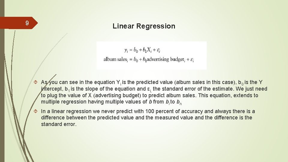
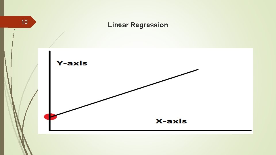
8 Linear Regression Linear regression is used when we want to ‘predict’ an outcome based on the manipulated conditions from the independent(s) variable(s). Regression is a step forward from correlation since with a good solid sample and design, we can predict outcome with the linear regression equation when the pure correlation will only show the strength of the correlation between two variables measures from -1 to + 1 (from a perfect negative linear relationship to a perfect positive relationship). This should never be confused with cause and effect since two variables can be highly correlated without one causing the other. It is worth to mention that on a solid and strong regression the correlation is implicit. We can have simple regression (One IV variable), multiple regression (Many IV variables) and Logistic regression where the outcome is dichotomous. “let’s look at an example. Imagine that I was interested in predicting physical and downloaded album sales (outcome) from the amount of money spent advertising that album (predictor). We could summarize this relationship using a linear model by replacing the names of our variables into equation (8. 1): Once we have estimated the values of the bs we would be able to make a prediction” (Field, 2013, p. 295)

9 Linear Regression As you can see in the equation Yi is the predicted value (album sales in this case), b 0 is the Y intercept, b 1 is the slope of the equation and εi, the standard error of the estimate. We just need to plug the value of X (advertising budget) to predict album sales. This equation, extends to multiple regression having multiple values of b from bi to bn. In a linear regression we never predict with 100 percent of accuracy and always there is a difference between the predicted value and the measured value and the difference is the standard error.

10 Linear Regression

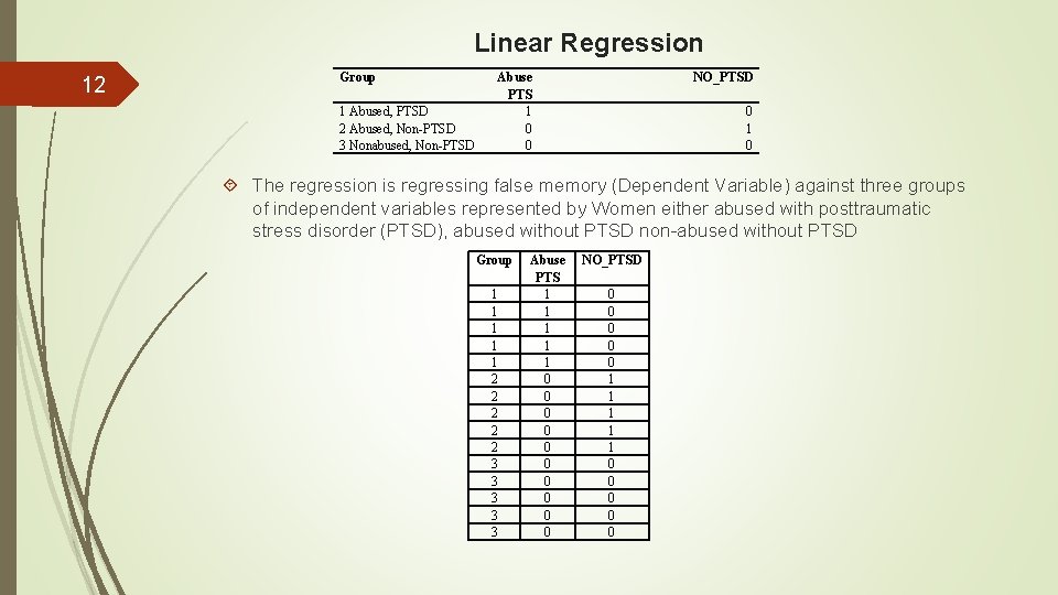
11 Linear Regression We can conduct linear regression with interval variables, categorical variables and a combination of both. To be able to use categorical variables on multiple regression we need to create N-1 dummy variables for the system to conduct the regression examining each variable with the other variables held constant. For example, if we have three groups that we want to use to run a multiple linear regression the below table shows the needed coding.

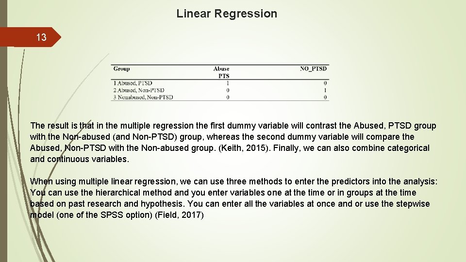
Linear Regression 12 Group 1 Abused, PTSD 2 Abused, Non-PTSD 3 Nonabused, Non-PTSD Abuse PTS 1 0 0 NO_PTSD 0 1 0 The regression is regressing false memory (Dependent Variable) against three groups of independent variables represented by Women either abused with posttraumatic stress disorder (PTSD), abused without PTSD non-abused without PTSD Group 1 1 1 2 2 2 3 3 3 Abuse PTS 1 1 1 0 0 0 0 0 NO_PTSD 0 0 0 1 1 1 0 0 0

Linear Regression 13 The result is that in the multiple regression the first dummy variable will contrast the Abused, PTSD group with the Non-abused (and Non-PTSD) group, whereas the second dummy variable will compare the Abused, Non-PTSD with the Non-abused group. (Keith, 2015). Finally, we can also combine categorical and continuous variables. When using multiple linear regression, we can use three methods to enter the predictors into the analysis: You can use the hierarchical method and you enter variables one at the time or in groups at the time based on past research and hypothesis. You can enter all the variables at once and or use the stepwise model (one of the SPSS option) (Field, 2017)

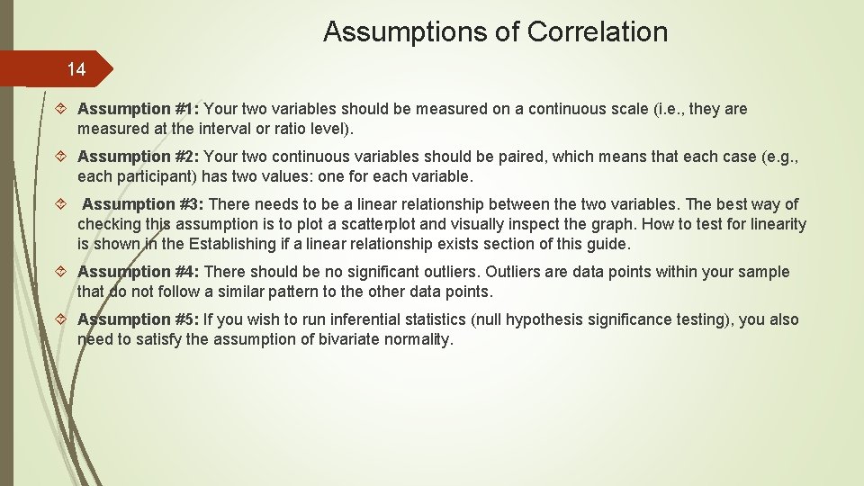
Assumptions of Correlation 14 Assumption #1: Your two variables should be measured on a continuous scale (i. e. , they are measured at the interval or ratio level). Assumption #2: Your two continuous variables should be paired, which means that each case (e. g. , each participant) has two values: one for each variable. Assumption #3: There needs to be a linear relationship between the two variables. The best way of checking this assumption is to plot a scatterplot and visually inspect the graph. How to test for linearity is shown in the Establishing if a linear relationship exists section of this guide. Assumption #4: There should be no significant outliers. Outliers are data points within your sample that do not follow a similar pattern to the other data points. Assumption #5: If you wish to run inferential statistics (null hypothesis significance testing), you also need to satisfy the assumption of bivariate normality.

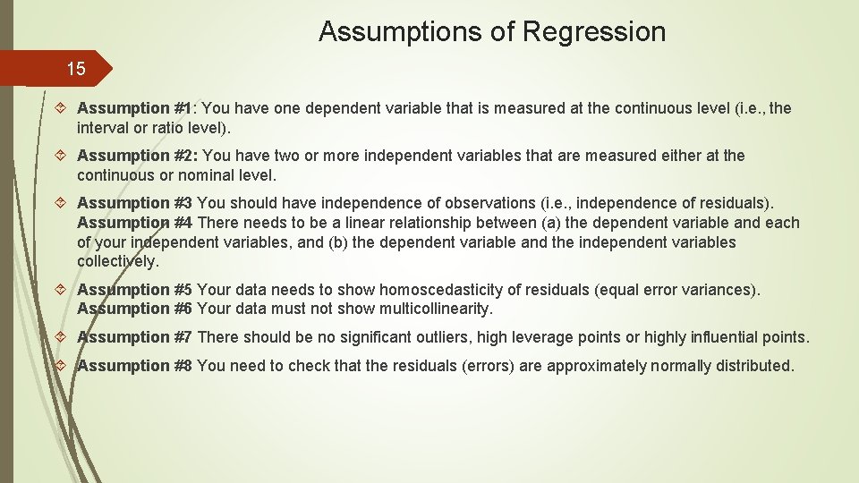
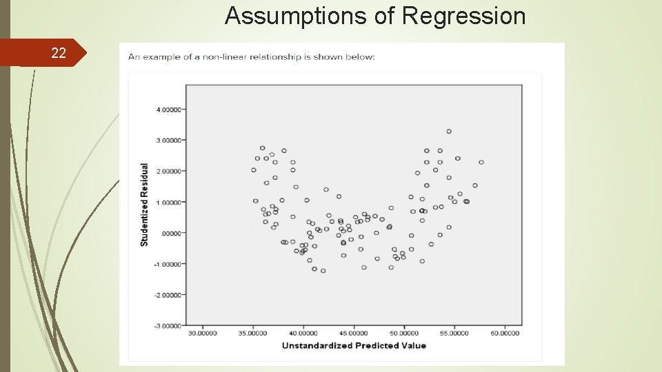
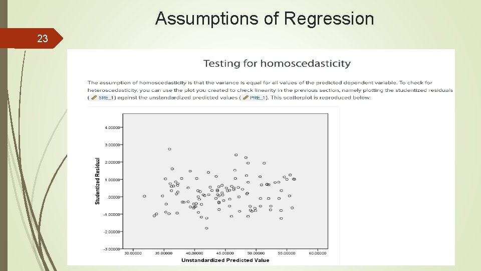
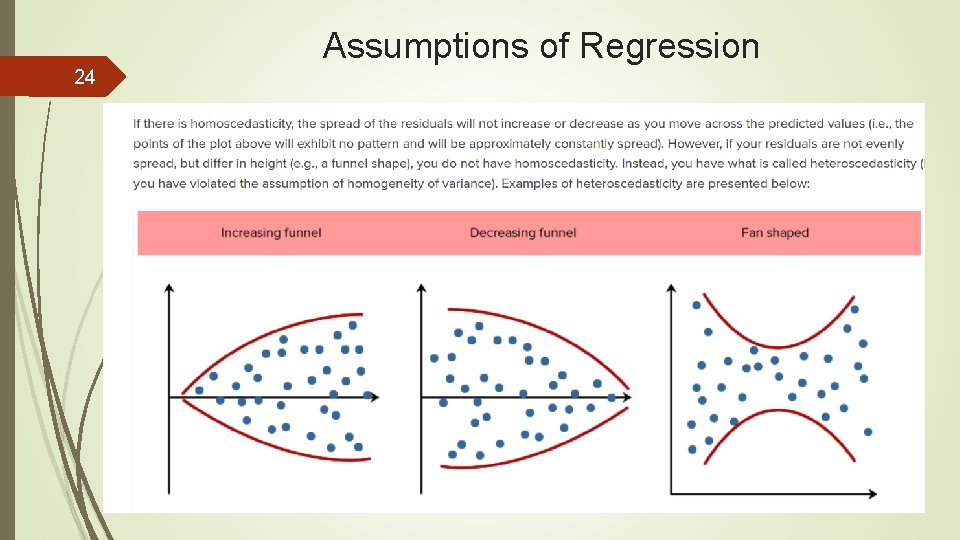
Assumptions of Regression 15 Assumption #1: You have one dependent variable that is measured at the continuous level (i. e. , the interval or ratio level). Assumption #2: You have two or more independent variables that are measured either at the continuous or nominal level. Assumption #3 You should have independence of observations (i. e. , independence of residuals). Assumption #4 There needs to be a linear relationship between (a) the dependent variable and each of your independent variables, and (b) the dependent variable and the independent variables collectively. Assumption #5 Your data needs to show homoscedasticity of residuals (equal error variances). Assumption #6 Your data must not show multicollinearity. Assumption #7 There should be no significant outliers, high leverage points or highly influential points. Assumption #8 You need to check that the residuals (errors) are approximately normally distributed.

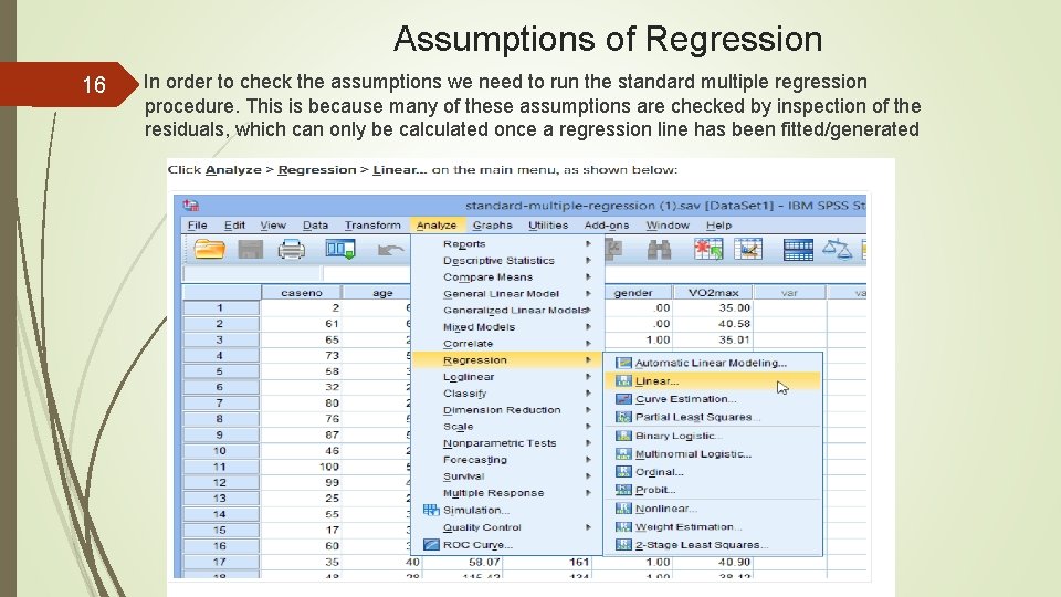
Assumptions of Regression 16 In order to check the assumptions we need to run the standard multiple regression procedure. This is because many of these assumptions are checked by inspection of the residuals, which can only be calculated once a regression line has been fitted/generated

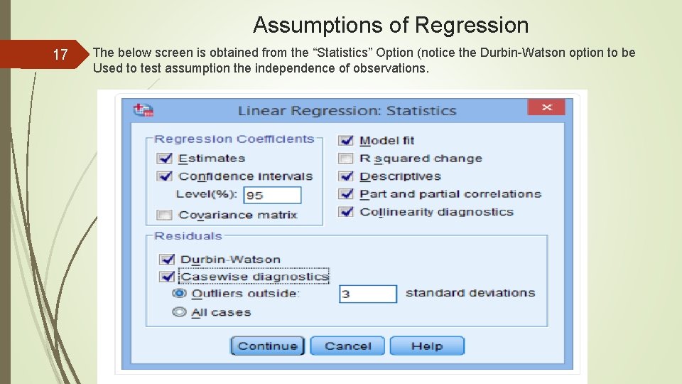
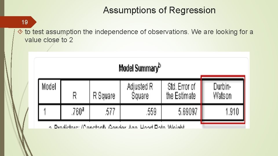
Assumptions of Regression 17 The below screen is obtained from the “Statistics” Option (notice the Durbin-Watson option to be Used to test assumption the independence of observations.

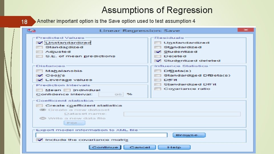
Assumptions of Regression 18 Another important option is the Save option used to test assumption 4

Assumptions of Regression 19 to test assumption the independence of observations. We are looking for a value close to 2

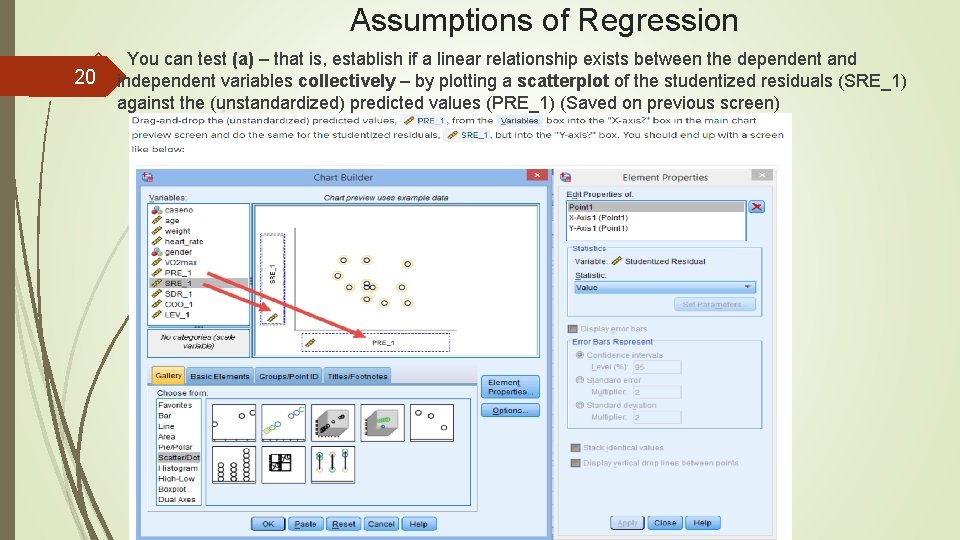
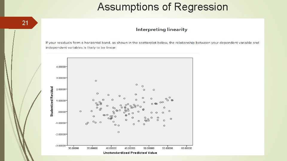
Assumptions of Regression 20 You can test (a) – that is, establish if a linear relationship exists between the dependent and independent variables collectively – by plotting a scatterplot of the studentized residuals (SRE_1) against the (unstandardized) predicted values (PRE_1) (Saved on previous screen)

Assumptions of Regression 21

Assumptions of Regression 22

Assumptions of Regression 23

Assumptions of Regression 24

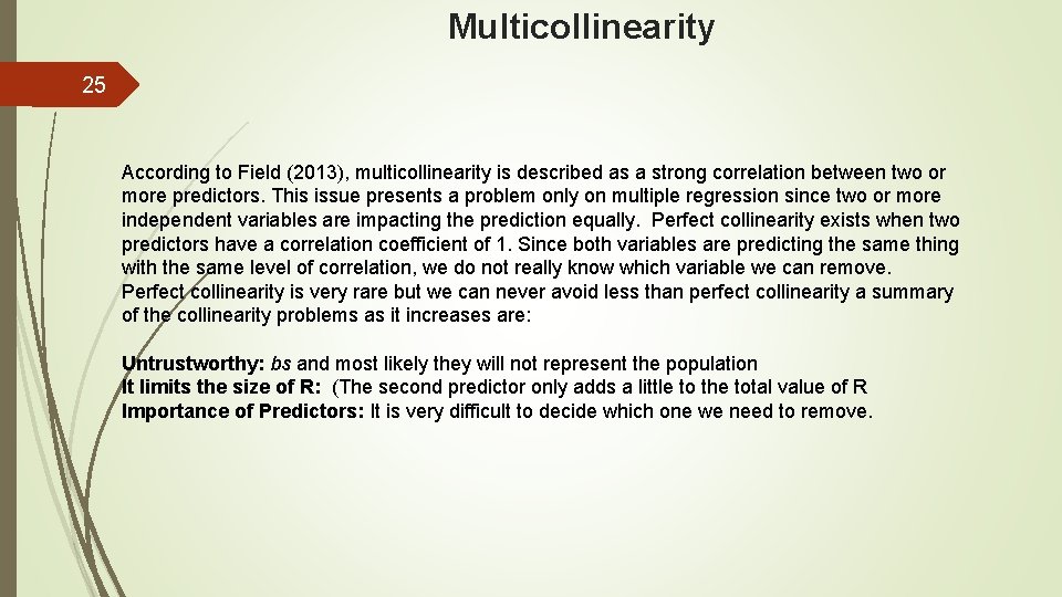
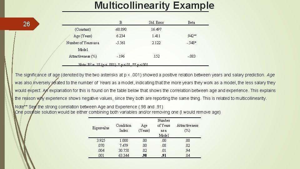
Multicollinearity 25 According to Field (2013), multicollinearity is described as a strong correlation between two or more predictors. This issue presents a problem only on multiple regression since two or more independent variables are impacting the prediction equally. Perfect collinearity exists when two predictors have a correlation coefficient of 1. Since both variables are predicting the same thing with the same level of correlation, we do not really know which variable we can remove. Perfect collinearity is very rare but we can never avoid less than perfect collinearity a summary of the collinearity problems as it increases are: Untrustworthy: bs and most likely they will not represent the population It limits the size of R: (The second predictor only adds a little to the total value of R Importance of Predictors: It is very difficult to decide which one we need to remove.

Multicollinearity Example 26 B Std. Error Beta (Constant) -60. 890 16. 497 Age (Years) 6. 234 1. 411 . 942** Number of Years as a -5. 561 2. 122 -. 548* -. 196 . 152 -. 083 Model Attractiveness (%) Note: R 2 =. 18 (p <. 001). * p <. 01, ** p <. 001 The significance of age (denoted by the two asterisks at p <. 001) showed a positive relation between years and salary prediction. Age was also inversely related to the number of Years as a model, indicating that the more years they work as a model, the less salary they would expect. An explanation for this is found on the table below that shows the correlation between age and experience. This explains the reason why experience shows negative values, since they both are reporting the same thing. This is related to multicollinearity. Note** See the strong correlation between Age and Experience (. 98 and. 91) One possible solution would be either combining both variables and/or removing one (I would remove age) Eigenvalue Condition Index Age (Years) 3. 925. 070. 004. 001 1. 000 7. 479 30. 758 63. 344 . 00. 02. 98 Number of Years as a Model. 00. 08. 01. 91 Attractiveness (%). 00. 02. 94. 04

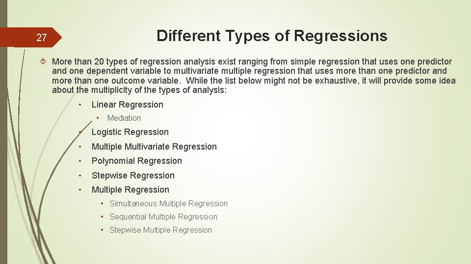
Different Types of Regressions 27 More than 20 types of regression analysis exist ranging from simple regression that uses one predictor and one dependent variable to multivariate multiple regression that uses more than one predictor and more than one outcome variable. While the list below might not be exhaustive, it will provide some idea about the multiplicity of the types of analysis: • Linear Regression • Mediation • Logistic Regression • Multiple Multivariate Regression • Polynomial Regression • Stepwise Regression • Multiple Regression • Simultaneous Multiple Regression • Sequential Multiple Regression • Stepwise Multiple Regression

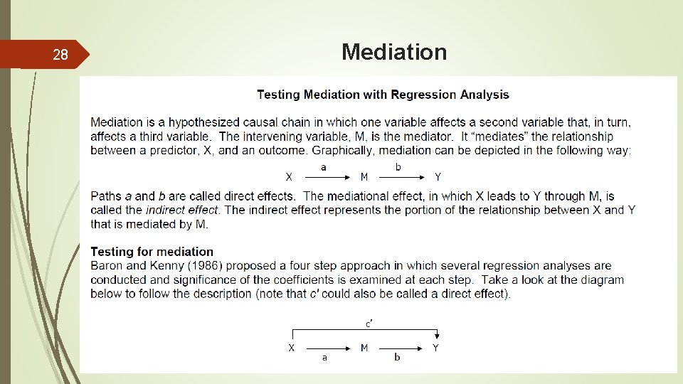
28 Mediation

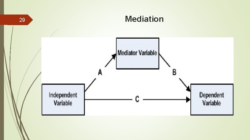
29 Mediation

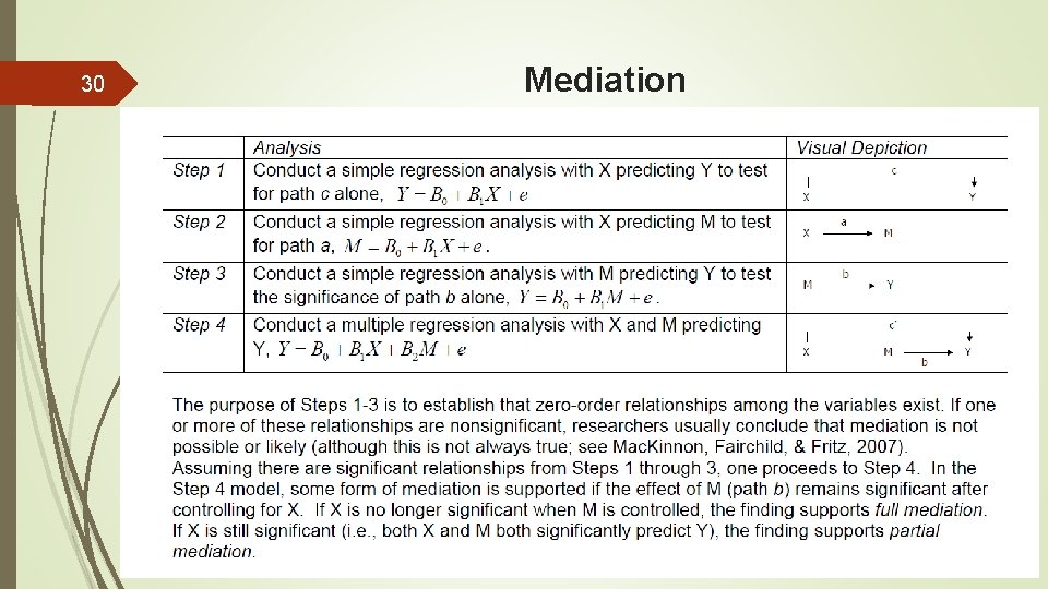
30 Mediation

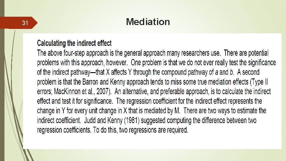
31 Mediation

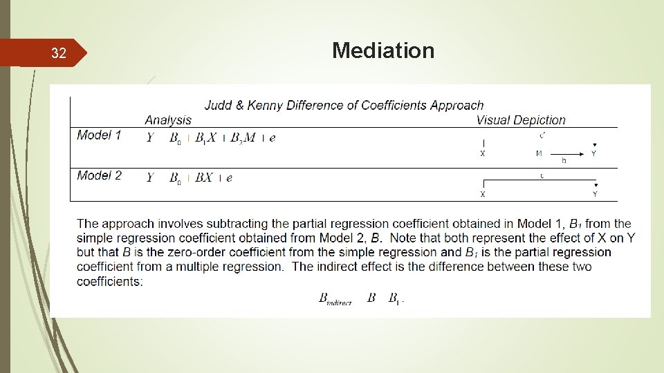
32 Mediation

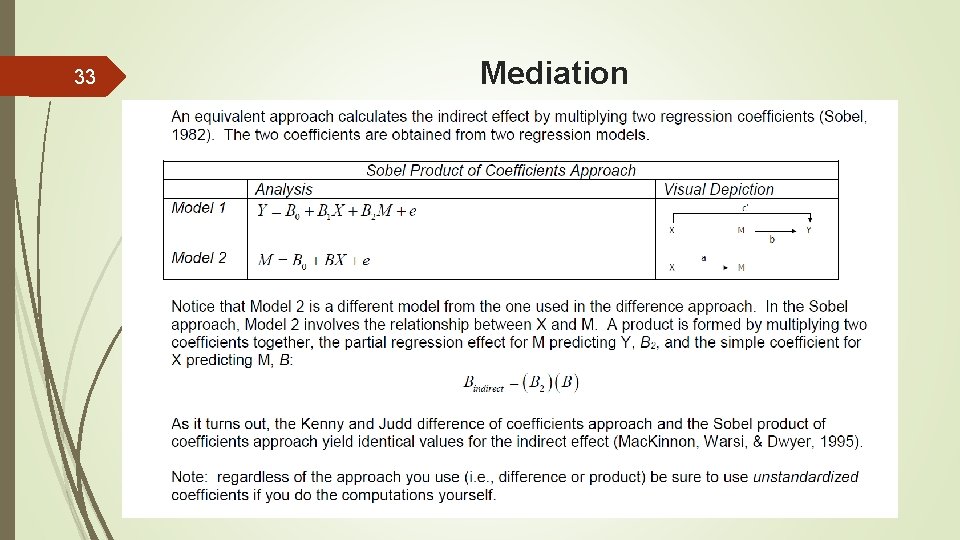
33 Mediation

34 Statistical tests of the indirect effect (Not Covered in this Presentation Bootstrap Method Monte Carlo Method SEM (Structural Equation Modeling)

References Bevins, T. (n. d. ). Research Designs. Retrieved from http: //ruby. fgcu. edu/courses/sbevins/50065/qtdesign. html 35 Cohen, J. , Cohen, P. , West, S. G. , & Aiken, L. S. (2003). Applied multiple correlation/regression analysis for the behavioral sciences. UK: Taylor & Francis. Coolican, H. (2014). Research methods and statistics in psychology. London: Psychology Press, Taylor & Francis Group. Field, A. (2017). Discovering statistics using IBM SPSS statistics. sage. Fraenkel, J. R. , Wallen, N. E. , & Hyun, H. H. (2016). How to design and evaluate research in education. Mc. Graw-Hill Education. Holton, E. F. , & Burnett, M. F. (2005). The basics of quantitative research. Research in organizations: Foundations and methods of inquiry, 29 -44. Iichaan. (2015, June 27). Weaknesses and Disadvantages of Causal Comparative Research Essay. Retrieved from http: //www. antiessays. com/free-essays/Weaknesses-And-Disadvantages-Of-Causal-Comparative-750679. html Keith, T. Z. (2014). Multiple regression and beyond: An introduction to multiple regression and structural equation modeling. Routledge. Miles, J. , & Shevlin, M. (2001). Applying regression and correlation: A guide for students and researchers. Sage. Nayak, B. , & Hazra, A. (2011). How to choose the right statistical test? Indian Journal of Ophthalmology, 59(2), 85. doi: 10. 4103/0301 -4738. 77005 Salkind, N. J. (Ed. ). (2010). Encyclopedia of research design (Vol. 1). Sage. Topchyan, R. (2013). Factors affecting knowledge sharing in virtual learning teams (VLTs) in distance education (Doctoral dissertation, Syracuse University). Testing Mediation with Regression Analysis. Retrieved from http: //web. pdx. edu/~newsomj/semclass/ho_mediation. pdf

Questions?