CORRELATION We have studied the major statistical proprties

CORRELATION

• We have studied the major statistical proprties we investigate in univariate data, i. e. data observed on a single variable. However, in practical situations, we consider several characteristics/variables( interval or scale type ) simultaneously. • Ex: age, height, weight, BP, blood sugar, cholesterol, mothers weight, weight of the new born baby, etc.

• Consider the pairs of variables: (height, weight) , ( age, weight ) , (weight , BP ) • How does weight vary with height? or what kind of association is shown between the two variables? • By association we mean the nature of change in the values of the two variables. Do they change in the same direction – both increase or both decrease together, or as one variable increases the other variable decreases?

• or no such association is found. • This kind of association existing between two variables is called correlation. • When the two variables are associated in the same direction, we say that they are positively correlated. If the association is in opposite directions , it is called negative correlation. • If the two variables do not show clear and consistent association , then they are uncorrelated.

Some examples • Degree of overcrowding and prevalence of pulmonary tuberculosis • Severity of malnutrition and prevalence of tuberculosis • Economic status and health status • Ageing and blood pressure

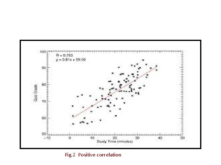
Understanding correlation graphically • The type of association between two variables can be graphically examined by plotting the values of one variable, say height ( X ) against weight ( Y ) in a graph. Such a plot is called scatter plot. • As height increases, if weight also increases ( it is so , generally ) then height and weight are positively correlated.

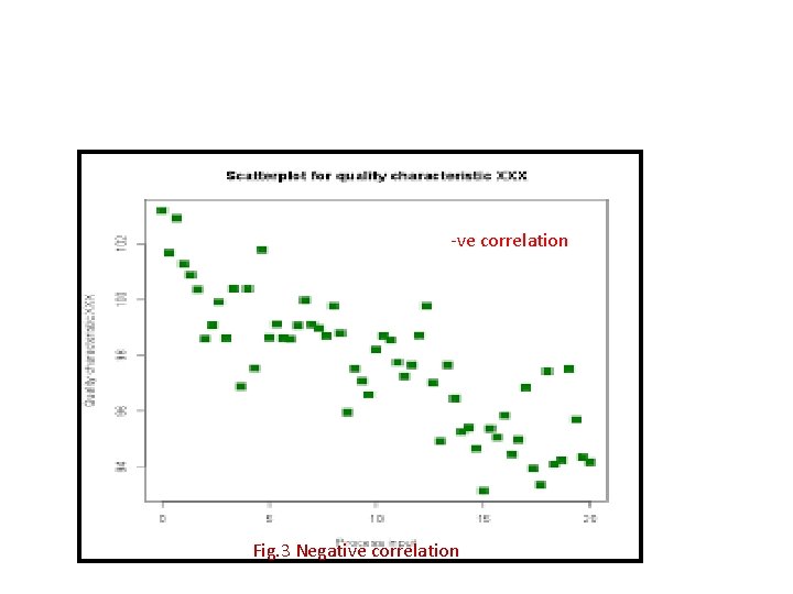
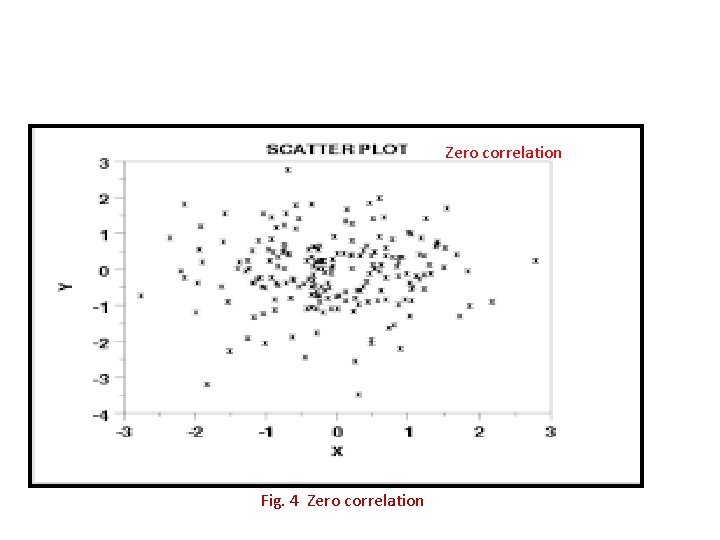
• As X increases Y decreases , then X and Y are negatively correlated. • If no such clear pattern of variation is found then there is no correlation or zero correlation.

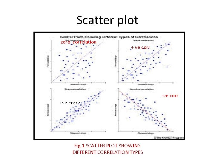
Scatter plot zero correlation + ve corr -ve corr +ve corre Fig. 1 SCATTER PLOT SHOWING DIFFERENT CORRELATION TYPES

Fig. 2 Positive correlation

-ve correlation Fig. 3 Negative correlation

Zero correlation Fig. 4 Zero correlation

How to use scatter plot? • If the points are forming an elliptic shape starting from the left bottom and ascending to the right top then the variables are positively correlated. ( Fig. 1 , Fig. 2 ) • If the points are forming an elliptic shape starting from the left top and descending to the right bottom then the variables are negatively correlated. ( Fig. 3 )

• If the points plotted do not show increasing or decreasing pattern but spread out in the scatter plot, then there is no correlation/zero correlation between the variables. • Presence of correlation between the two variables is indicative of possible linear relationship between the two variables. • Hence some authors/books call it ‘ linear correlation ‘

Measurement of correlation • Scatter plot is useful to identify the type/nature of correlation. A quantitative measure of correlation between two variables is correlation coefficient. • Karl Pearson’s Product Moment Correlation Coefficient ( or simply Pearson’s correlation coefficient ) is one such measure.

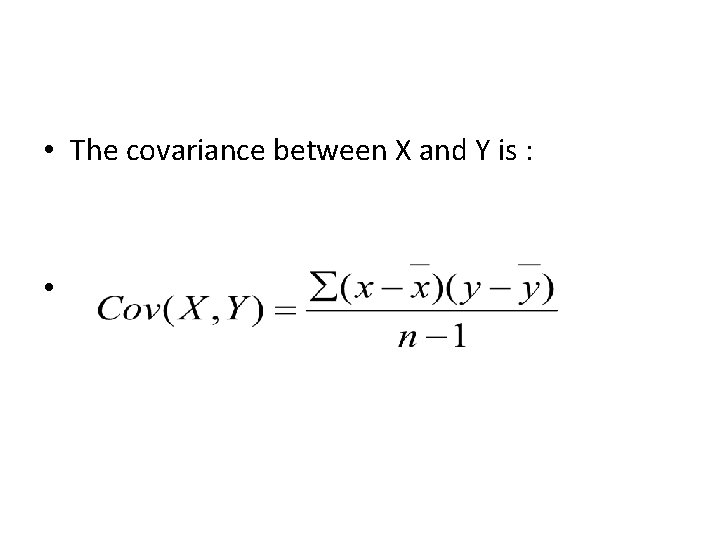
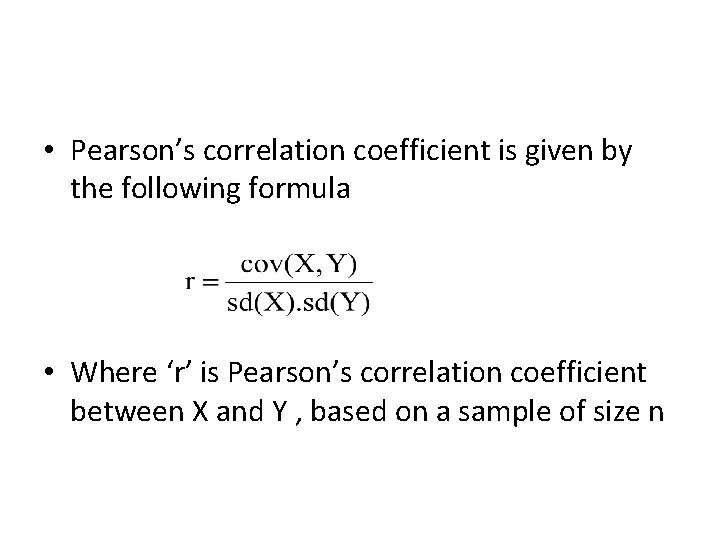
• Pearson’s correlation coefft. tells us how much one variable changes as the values of another changes – their covariation. • Covariation is measured by calculating the amount by which each value of X varies from the mean of X, and the amount by which each value of Y varies from the mean of Y and multiplying the differences together and finding the average ( dividing by (n-1) in case of sample. ). This is called covariance between X and Y.

• The covariance between X and Y is : •

• Pearson’s correlation coefficient is given by the following formula • Where ‘r’ is Pearson’s correlation coefficient between X and Y , based on a sample of size n

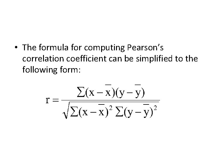
• The formula for computing Pearson’s correlation coefficient can be simplified to the following form:

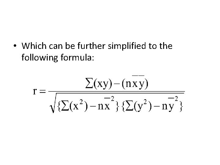
• Which can be further simplified to the following formula:

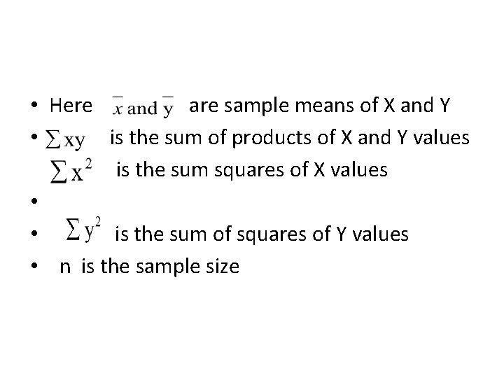
• Here are sample means of X and Y • is the sum of products of X and Y values is the sum squares of X values • • is the sum of squares of Y values • n is the sample size

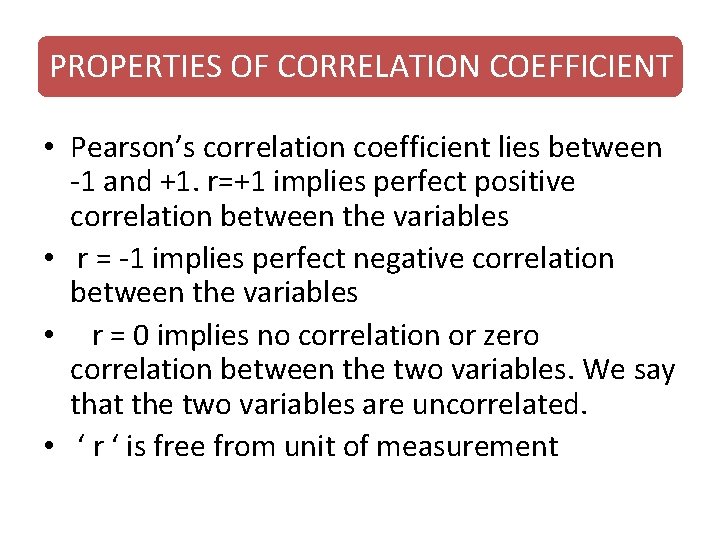
PROPERTIES OF CORRELATION COEFFICIENT • Pearson’s correlation coefficient lies between -1 and +1. r=+1 implies perfect positive correlation between the variables • r = -1 implies perfect negative correlation between the variables • r = 0 implies no correlation or zero correlation between the two variables. We say that the two variables are uncorrelated. • ‘ r ‘ is free from unit of measurement

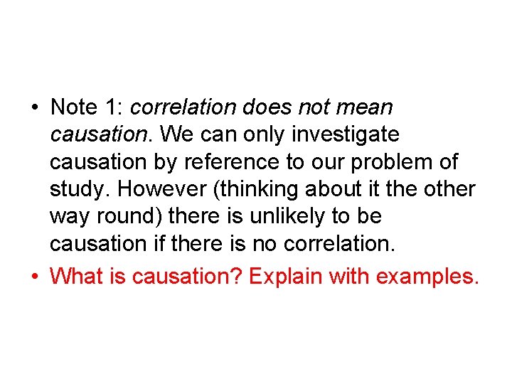
• Note 1: correlation does not mean causation. We can only investigate causation by reference to our problem of study. However (thinking about it the other way round) there is unlikely to be causation if there is no correlation. • What is causation? Explain with examples.

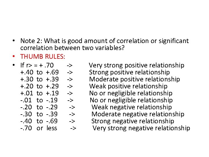
• Note 2: What is good amount of correlation or significant correlation between two variables? • THUMB RULES: • If r> = +. 70 -> Very strong positive relationship +. 40 to +. 69 -> Strong positive relationship +. 30 to +. 39 -> Moderate positive relationship +. 20 to +. 29 -> Weak positive relationship +. 01 to +. 19 -> No or negligible relationship -. 01 to -. 19 -> No or negligible relationship -. 20 to -. 29 -> Weak negative relationship -. 30 to -. 39 -> Moderate negative relationship -. 40 to -. 69 -> Strong negative relationship -. 70 or less -> Very strong negative relationship

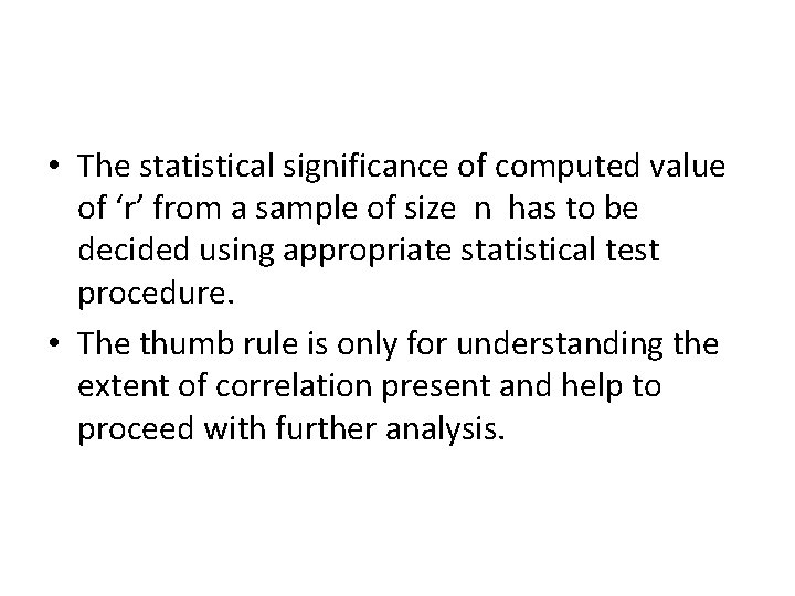
• The statistical significance of computed value of ‘r’ from a sample of size n has to be decided using appropriate statistical test procedure. • The thumb rule is only for understanding the extent of correlation present and help to proceed with further analysis.

Some precautions • The two variables of interest are measured on the same entity. If we consider height and weight, these two variables are measured on the same individual. It does not make sense to speak of the correlation between the heights of one group of individuals and the weights of another group.

• No matter how strong is the correlation between two variables , it should not be interpreted as one of cause and effect. A significant correlation between X and Y may mean: • X causes Y • Y causes X • Some third factor inducing association between X and Y • The correlation could be ‘spurious’ or ‘nonsensical’

For self learning……… • When data are given in the form of grouped bivariate with frequency values how to compute correlation coefficient? • Learn from text books or other sources. • Since in most of the cases data are organised in computer files and calculation is done using statistical packages, the above situation does not arise.

SPEARMAN’S RANK CORRELATION • Spearman's rank correlation coefficient or Spearman's rho, named after Charles Spearman and often denoted by the Greek letter ρ , is a nonparametric measure of statistical dependence between two variables. • Spearman rank correlation measures the association between two ranked variables, or one ranked variable and one measurement variable. You can also use Spearman rank correlation instead of Pearson’s correlation for two measurement variables if you're worried about non-normality, but this is not usually necessary.

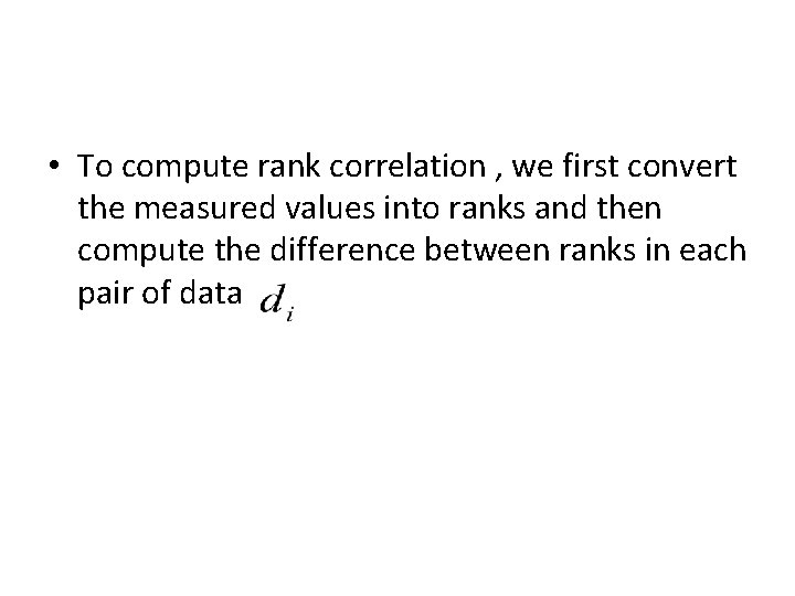
• To compute rank correlation , we first convert the measured values into ranks and then compute the difference between ranks in each pair of data

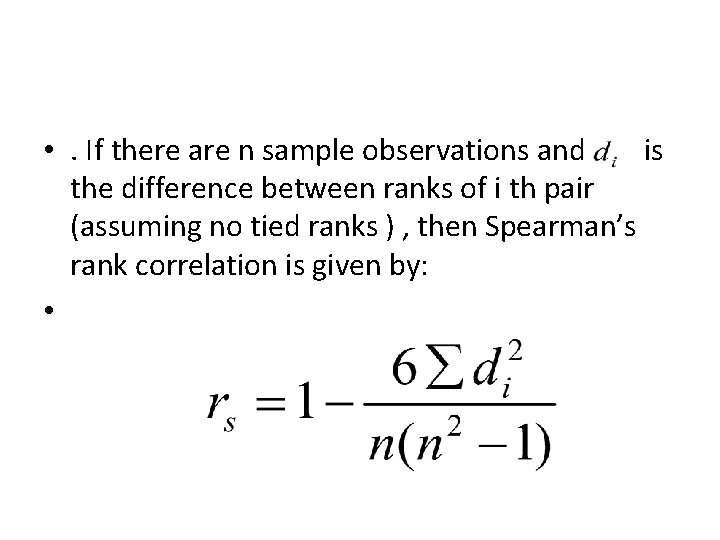
• . If there are n sample observations and is the difference between ranks of i th pair (assuming no tied ranks ) , then Spearman’s rank correlation is given by: •

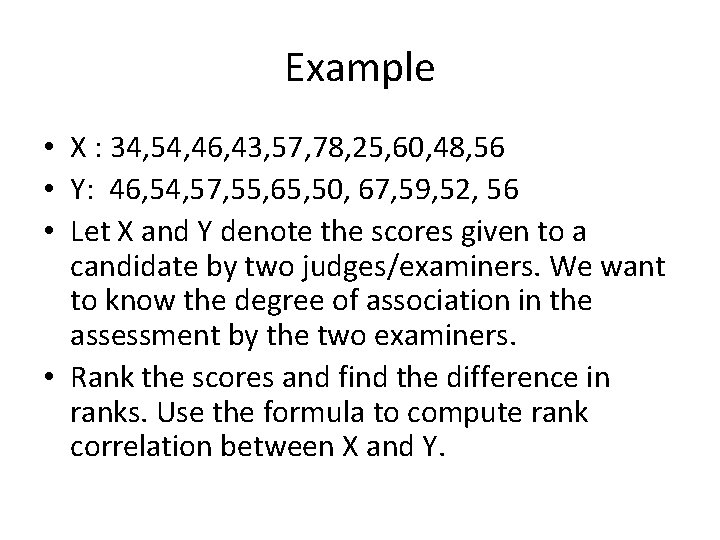
Example • X : 34, 54, 46, 43, 57, 78, 25, 60, 48, 56 • Y: 46, 54, 57, 55, 65, 50, 67, 59, 52, 56 • Let X and Y denote the scores given to a candidate by two judges/examiners. We want to know the degree of association in the assessment by the two examiners. • Rank the scores and find the difference in ranks. Use the formula to compute rank correlation between X and Y.