Correlation How Strong Is the Linear Relationship Lecture
- Slides: 30

Correlation: How Strong Is the Linear Relationship? Lecture 50 Sec. 13. 7 Fri, Apr 22, 2005

The Correlation Coefficient The correlation coefficient r is a number between – 1 and +1. n It measures the direction and strength of the linear relationship. n If r > 0, then the relationship is positive. If r < 0, then the relationship is negative. n The closer r is to +1 or – 1, the stronger the relationship. n The closer r is to 0, the weaker the relationship. n

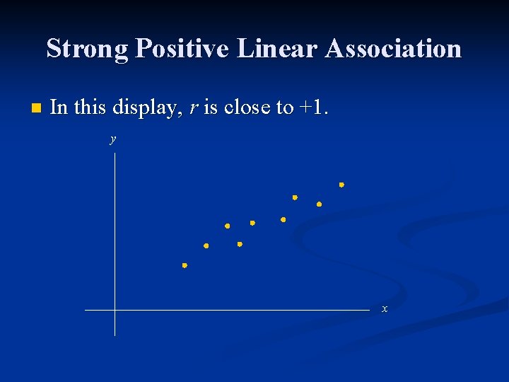
Strong Positive Linear Association n In this display, r is close to +1. y x

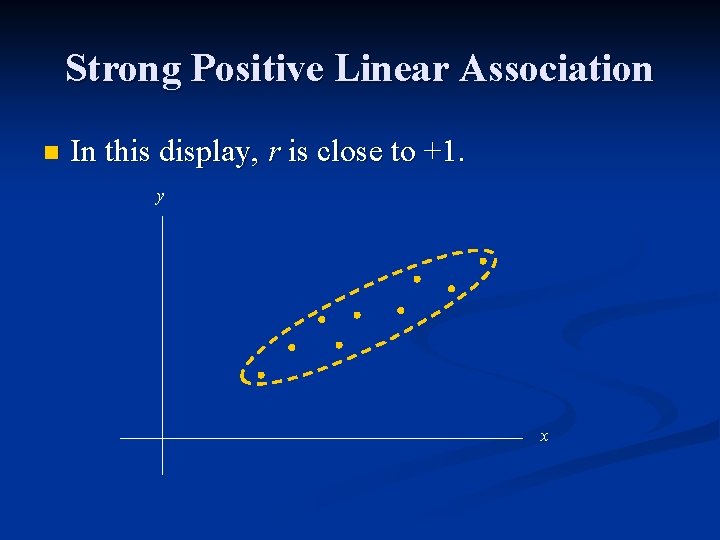
Strong Positive Linear Association n In this display, r is close to +1. y x

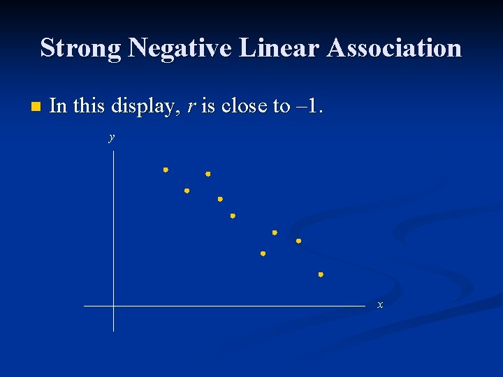
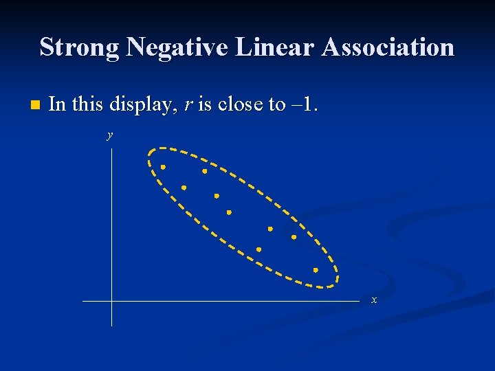
Strong Negative Linear Association n In this display, r is close to – 1. y x

Strong Negative Linear Association n In this display, r is close to – 1. y x

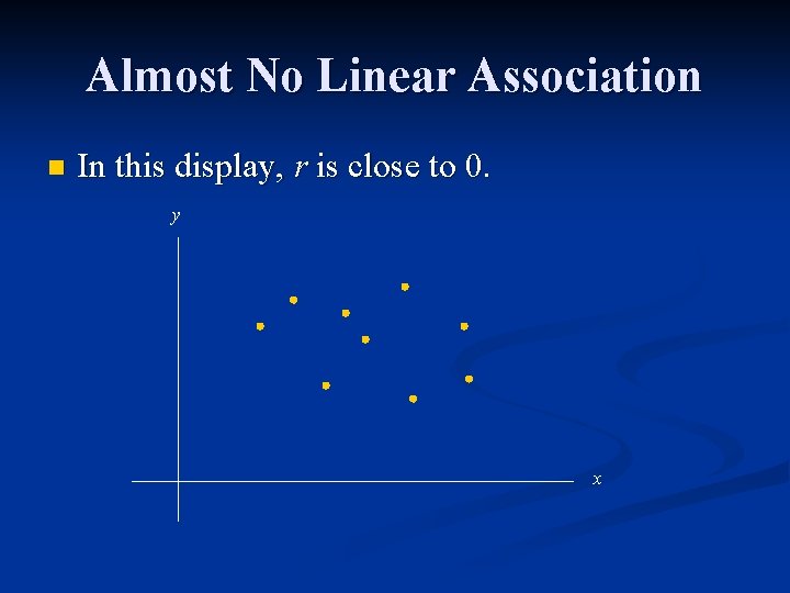
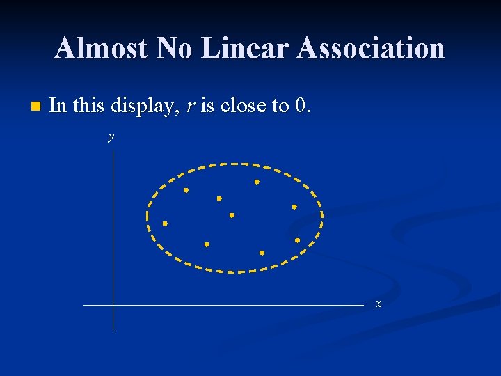
Almost No Linear Association n In this display, r is close to 0. y x

Almost No Linear Association n In this display, r is close to 0. y x

Correlation vs. Cause and Effect If the value of r is close to +1 or -1, that indicates that x is a good predictor of y. n It does not indicate that x causes y. n The correlation coefficient cannot be used to determine cause and effect. n

Correlation vs. Cause and Effect There is good reason to believe that the size of a person’s waistline is a predictor of his performance on an algebra test (within the age range 0 – 21). n However, increasing your waistline will not help you on an algebra test. n Conversely, learning more algebra will not increase your waistline. n So why is there a relationship? n

“Third” Variables The hidden third variable is age. n Age causes (to some extent) the waistline to increase. n Age causes (to some extent) a person to do better on an algebra test. n

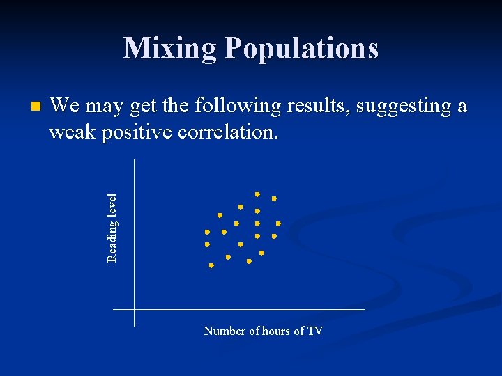
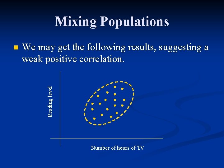
Mixing Populations Mixing nonhomogeneous groups can create a misleading correlation coefficient. n Suppose we gather data on the number of hours spent watching TV each week and the child’s reading level, for 1 st, 2 nd, and 3 rd grade students. n

Mixing Populations We may get the following results, suggesting a weak positive correlation. Reading level n Number of hours of TV

Mixing Populations We may get the following results, suggesting a weak positive correlation. Reading level n Number of hours of TV

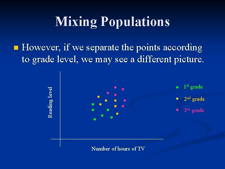
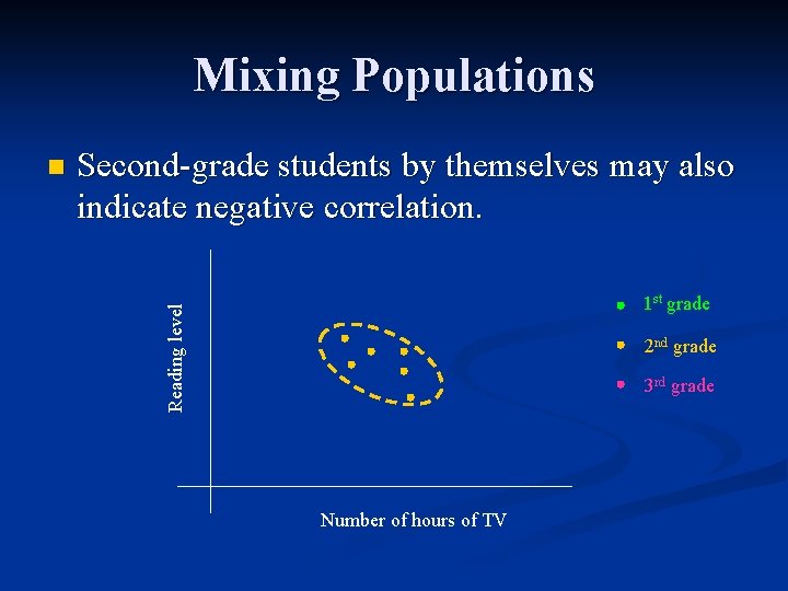
Mixing Populations However, if we separate the points according to grade level, we may see a different picture. 1 st grade Reading level n 2 nd grade 3 rd grade Number of hours of TV

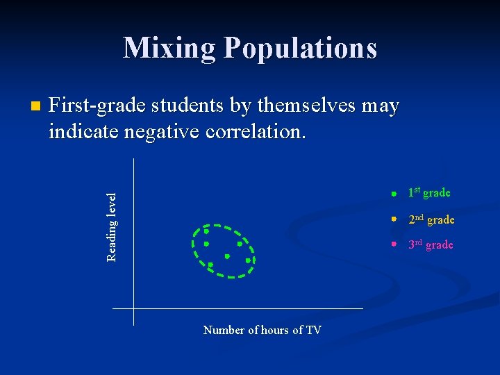
Mixing Populations First-grade students by themselves may indicate negative correlation. 1 st grade Reading level n 2 nd grade 3 rd grade Number of hours of TV

Mixing Populations Second-grade students by themselves may also indicate negative correlation. 1 st grade Reading level n 2 nd grade 3 rd grade Number of hours of TV

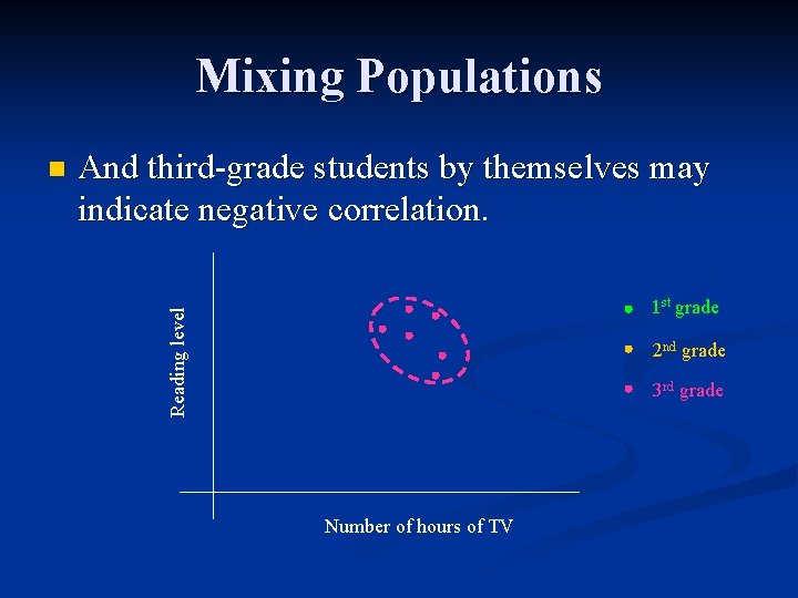
Mixing Populations And third-grade students by themselves may indicate negative correlation. 1 st grade Reading level n 2 nd grade 3 rd grade Number of hours of TV

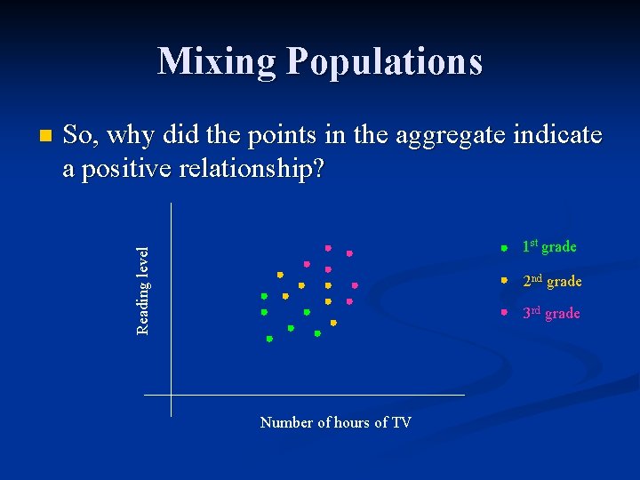
Mixing Populations So, why did the points in the aggregate indicate a positive relationship? 1 st grade Reading level n 2 nd grade 3 rd grade Number of hours of TV

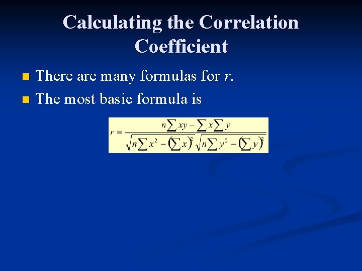
Calculating the Correlation Coefficient There are many formulas for r. n The most basic formula is n

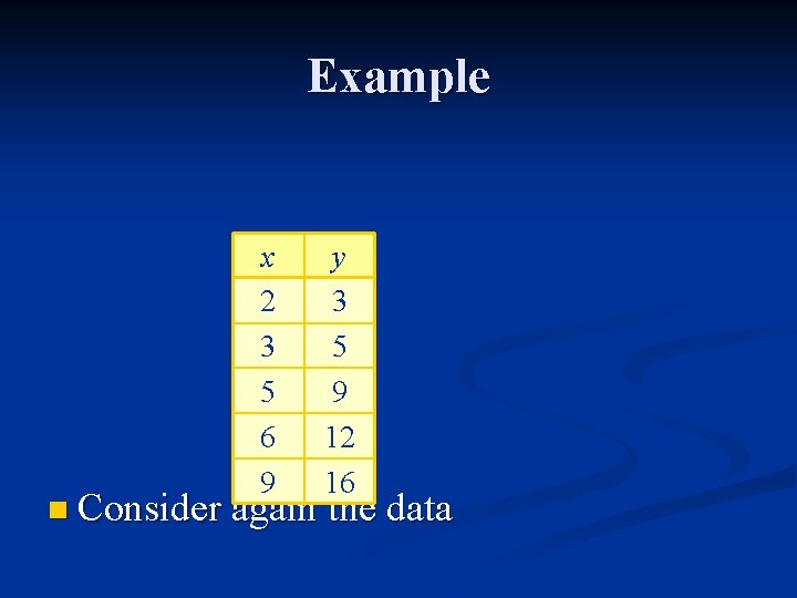
Example x 2 3 5 6 9 y 3 5 9 12 16 n Consider again the data

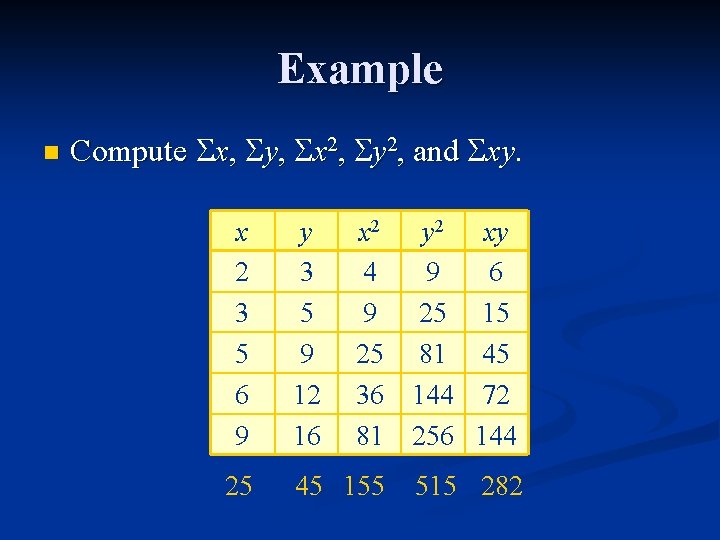
Example n Compute x, y, x 2, y 2, and xy. xy x 2 3 5 6 9 25 y 3 5 9 12 16 x 2 4 9 25 36 81 y 2 xy 9 6 25 15 81 45 144 72 256 144 45 155 515 282

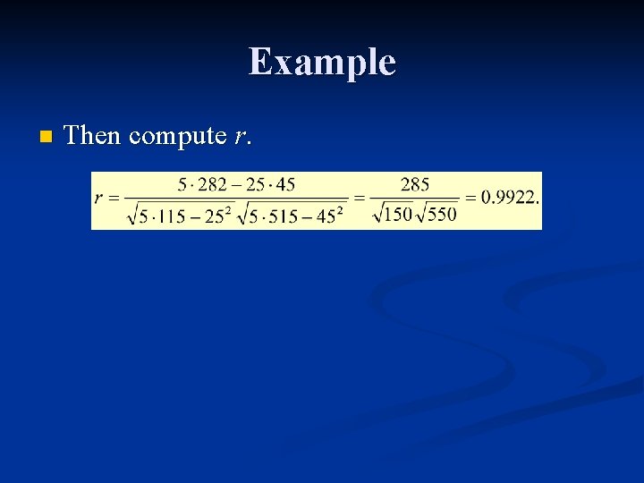
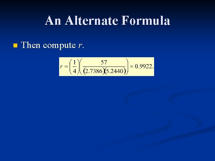
Example n Then compute r.

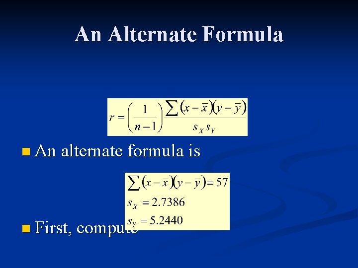
An Alternate Formula n An alternate formula is n First, compute

An Alternate Formula n Then compute r.

TI-83 – Calculating r n To calculate r on the TI-83, First, be sure that Diagnostic is turned on. n Then, follow the procedure that produces the regression line. n In the same window, the TI-83 reports r 2 and r. n n Use the TI-83 to calculate r in the preceding example.

Let’s Do It! n Let’s Do It! 13. 10, p. 781 – Oil-Change Data. n n Do part (b) on the TI-83. Let’s Do It! 13. 11, p. 782 – Data on Milk Production.

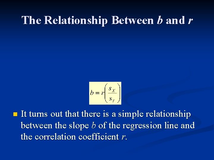
The Relationship Between b and r n It turns out that there is a simple relationship between the slope b of the regression line and the correlation coefficient r.

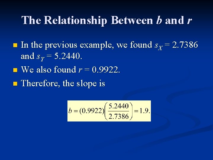
The Relationship Between b and r In the previous example, we found s. X = 2. 7386 and s. Y = 5. 2440. n We also found r = 0. 9922. n Therefore, the slope is n

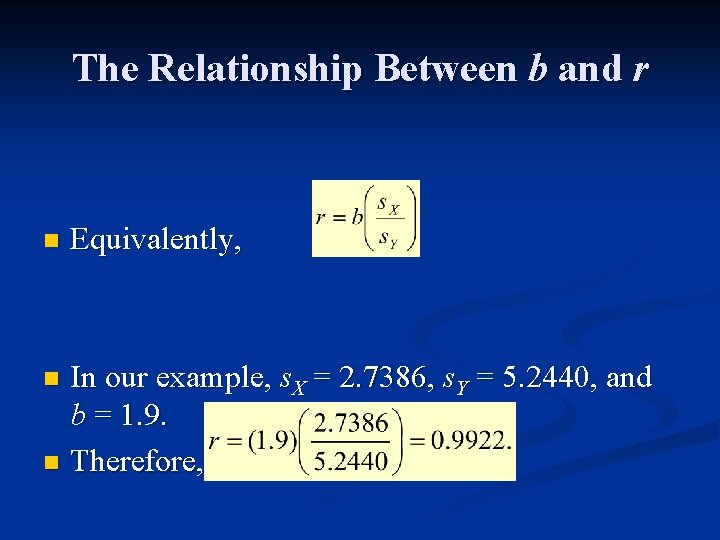
The Relationship Between b and r n Equivalently, In our example, s. X = 2. 7386, s. Y = 5. 2440, and b = 1. 9. n Therefore, n