CORRELATION Flow of Presentation Definition Types of correlation

CORRELATION

Flow of Presentation • Definition • Types of correlation • Method of studying correlation a) Scatter diagram b) Karl Pearson’s coefficient of correlation c) Spearman’s Rank correlation coefficient

Correlation • Correlation: The degree of relationship between the variables under consideration is measure through the correlation analysis. • The measure of correlation called the correlation coefficient. • The degree of relationship is expressed by coefficient which range from correlation ( -1 ≤ r ≥ +1) • The direction of change is indicated by a sign. • The correlation analysis enable us to have an idea about the degree & direction of the relationship between the two variables under study.

Correlation & Causation • Causation means cause & effect relation. • Correlation denotes the interdependency among the variables for correlating two phenomenon, it is essential that the two phenomenon should have cause-effect relationship, & if such relationship does not exist then the two phenomenon can not be correlated. • If two variables vary in such a way that movement in one are accompanied by movement in other, these variables are called cause and effect relationship. • Causation always implies correlation but correlation does not necessarily implies causation.

Types of Correlation Type I: Direction of the Correlation Positive Correlation Negative Correlation

Examples: • Positive relationships • Negative relationships: relationships Øalcohol consumption and Øwater consumption driving ability. and temperature. Østudy time and grades. ØPrice & quantity demanded

Type II: No of variables considered Correlation Simple Multiple Partial Total

Type III: Relationship assumed Correlation LINEAR NON LINEAR

Types of Correlation Type III • Linear correlation: Correlation is said to be linear when the amount of change in one variable tends to bear a constant ratio to the amount of change in the other. The graph of the variables having a linear relationship will form a straight line. Ex X = 1, 2, 3, 4, 5, 6, 7, 8, Y = 5, 7, 9, 11, 13, 15, 17, 19, Y = 3 + 2 x • Non Linear correlation: The correlation would be non linear if the amount of change in one variable does not bear a constant ratio to the amount of change in the other variable.

Methods of Studying Correlation • Scatter Diagram Method • Karl Pearson’s Coefficient of Correlation • Spearman’s Rank Correlation Coefficient

Scatter Diagram Method Scatter Diagram is a graph of observed plotted points where each points represents the values of X & Y as a coordinate. It portrays the relationship between these two variables graphically.

A perfect positive correlation Weight of B A linear relationship Weight of A Height of B Height

High Degree of positive correlation • Positive relationship r = +. 80 Weight Height

Degree of correlation • Moderate Positive Correlation r = + 0. 4 Shoe Size Weight

Degree of correlation • Perfect Negative Correlation r = -1. 0 TV watching per week Exam score

Degree of correlation • Moderate Negative Correlation r = -. 80 TV watching per week Exam score

Degree of correlation • Weak negative Correlation Shoe Size r = - 0. 2 Weight

Degree of correlation • No Correlation (horizontal line) r = 0. 0 IQ Height

Degree of correlation (r) r = +. 80 r = +. 60 r = +. 40 r = +. 20

Advantages and Disadvantage of Scatter Diagram Advantages: • Simple & Non Mathematical method • Not influenced by the size of extreme item • First step in investing the relationship between two variables Disadvantage: • Can not adopt the an exact degree of correlation

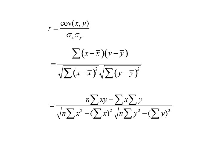
Karl Pearson's Coefficient of Correlation • Pearson’s ‘r’ is the most common correlation coefficient. • The coefficient of correlation ‘r’ measure the degree of linear relationship between two variables say x & y.

Karl Pearson’s Coefficient of Correlation denoted by- r Ø -1 ≤ r ≥ +1 Ø Degree of Correlation is expressed by a value of Coefficient Ø Direction of change is Indicated by sign ( - ve) or ( + ve) Ø

(r) Interpretation of Correlation Coefficient • The value of correlation coefficient ‘r’ ranges from -1 to +1 • If r = +1, then the correlation between the two variables is said to be perfect and positive • If r = -1, then the correlation between the two variables is said to be perfect and negative • If r = 0, then there exists no correlation between the variables

Properties of Correlation coefficient • The correlation coefficient lies between -1 & +1 symbolically ( - 1≤ r ≥ 1 ) • The correlation coefficient is independent of the change of origin & scale.

Assumptions of Pearson’s Correlation Coefficient • There is linear relationship between two variables, i. e. when the two variables are plotted on a scatter diagram a straight line will be formed by the points. • Cause and effect relation exists between different forces operating on the item of the two variable series.

Example: Find the correlation coefficient using Karl Pearson’s method for the following data. x 6 2 10 4 8 y 9 11 5 8 7

Solution: X 6 2 10 4 8 Y 9 11 5 8 7 XY 54 22 50 32 56 X*X 36 4 100 16 64 Y*Y 81 121 25 64 49 30 40 214 220 340

Advantages of Pearson’s Coefficient • It summarizes in one value, the degree of correlation & direction of correlation also.

Limitation of Pearson’s Coefficient • Always assume linear relationship • Interpreting the value of r is difficult. • Value of Correlation Coefficient is affected by the extreme values. • Time consuming methods

Coefficient of Determination • The convenient way of interpreting the value of correlation coefficient is to use of square of coefficient of correlation which is called Coefficient of Determination. • The Coefficient of Determination = r 2. • Suppose: r = 0. 9, r 2 = 0. 81 this would mean that 81% of the variation in the dependent variable has been explained by the independent variable.

Example: • Suppose: r = 0. 60 r = 0. 30 It does not mean that the first correlation is twice as strong as the second the ‘r’ can be understood by computing the value of r 2. When r = 0. 60 r 2 = 0. 36 -----(1) r = 0. 30 r 2 = 0. 09 -----(2) This implies that in the first case 36% of the total variation is explained whereas in second case 9% of the total variation is explained.

Spearman’s Rank Coefficient of Correlation • When statistical series in which the variables under study are not capable of quantitative measurement but can be arranged in serial order, in such situation Pearson’s correlation coefficient can not be used in such case Spearman Rank correlation can be used.

Interpretation of Rank Correlation Coefficient (R) • The value of rank correlation coefficient, R ranges from 1 to +1 • If R = +1, then there is complete agreement in the order of the ranks and the ranks are in the same direction • If R = -1, then there is complete agreement in the order of the ranks and the ranks are in the opposite direction • If R = 0, then there is no correlation

Rank Correlation Coefficient (R) • Equal Ranks or tie in Ranks: In such cases average ranks should be assigned to each individual. m = The number of time an item is repeated

Example: Find the Spearman’s rank correlation coefficient for the following data x 39 65 62 90 82 75 25 98 36 78 y 47 53 58 86 62 68 60 91 51 84

Solution: X y Rx Ry D D*D 39 47 8 10 -2 4 65 53 6 8 -2 4 62 58 7 7 0 0 90 86 2 2 0 0 82 62 3 5 -2 4 75 68 5 4 1 1 25 60 10 6 4 16 98 91 1 1 0 0 36 51 9 9 0 0 78 84 4 3 1 1

Exp. 2: • A physiologist wants to compare two methods A and B of teaching. He selected a random sample of 22 students. He grouped them into 11 pairs have approximately equal scores in an intelligence test. In each pair one student was taught by method A and the other by method B and examined after the course. The marks obtained by them as follows Pair 1 2 3 4 5 6 7 8 9 10 11 A 24 29 19 14 30 19 27 30 20 28 11 B 37 35 16 26 23 27 19 20 16 11 21

Solution: A 24 29 19 B 37 35 16 R_A 6 3 8. 5 R_B 1 2 9. 5 D 5 1 -1 D*D 25 1 1 14 30 19 27 30 20 28 11 26 23 27 19 20 16 11 21 10 1. 5 8. 5 5 1. 5 7 4 11 4 5 3 8 7 9. 5 11 6 6 -3. 5 5. 5 -3 -5. 5 -2. 5 -7 5 36 12. 25 30. 25 9 30. 25 6. 25 49 25

Advantages of Spearman’s Rank Correlation • This method is simpler to understand easier to apply compared to Karl Pearson’s correlation method. • This method is useful where we can give the ranks and not the actual data. (qualitative term) • This method is to use where the initial data in the form of ranks.

Disadvantages of Spearman’s Correlation • Cannot be used for finding out correlation in a grouped frequency distribution. • This method should be applied where N exceeds 30.

Advantages of Correlation studies • Show the amount (strength) of relationship present • Can be used to make predictions about the variables under study. • Can be used in many places, including natural settings, libraries, etc. • Easier to collect co relational data

Thanks