Correlation and Regression 1 Another area of inferential

Correlation and Regression 1

§ Another area of inferential statistics involves determining whether a relationship exists between two or more numerical or quantitative variables. § Is there a relationship between age and blood pressure? § Is there a relationship between birth weight and life span? § Is there a relationship between volume of sales and amount of advertising? 2

§ Correlation is a statistical method used to determining whether a relationship between variables exists. § Regression is a statistical method used to describe the nature of the relationship between variables, that is, positive or negative, linear or nonlinear. 3

1. Are two or more variables related? 2. If so, what is the strength of the relationship? 3. What type of relationship exists? 4. What kind of predictions can be made from this relationship? § To answer the first two questions, statisticians use a numerical measure called the correlation coefficient. § To answer the third question, you must ascertain whether the relationship is simple or multiple. 4

Simple Multiple § Two variables – independent § Multiple Regression and dependent § Simple relationship analysis is called Simple Regression – one independent variable is used to predict the dependent variable § Two or more independent variables are used to predict the dependent variable § Positive relationship=both increase/decrease § Negative relationship=one increases as the other decreases 5

§ In simple correlation and regression studies, the researcher collects data on two numerical or quantitative variables to see whether a relationship exists between the variables. § For example, if the researcher wanted to see if there was a relationship between number of hours of study and test scores on an exam, she must collect a random sample of students, determine the number of hours of study, and obtain their grades on the exam. A table can be made for the data, as shown here: Student Hours of Study x Grade y A 6 82 B 2 63 C 1 57 D 5 88 E 2 68 F 3 75 6

§ As previously stated, the two variables for this study are called independent and dependent. § Independent – can be controlled or manipulated (hours of study) § Dependent – cannot be controlled or manipulated (grade) § The determination of the x and y variables is not always clear-cut and is sometimes an arbitrary decision. § For example, if the researcher studies the effects of age on a person’s blood pressure, the researcher can generally assume that age affects blood pressure. § On the other hand, if a researcher is studying the attitudes of husbands on a certain issue and the attitudes of their wives on the same issue, it is difficult to say which variable is independent and which is dependent. Thus the researcher can arbitrarily designate the variables as independent and dependent. 7

§ The independent and dependent variables can be plotted on a graph called a scatter plot. § independent – x § dependent – y § A Scatter Plot is a graph of the ordered pairs (x, y) of numbers consisting of the independent variable x and the dependent variable y. § Used as a visual way to describe the nature of the relationship between the independent and dependent variables. 8

§ Make scatter plots of the following data to determine if there is a relationship between the two variables. Company Cars (in thousands) Revenue (in billions) A 63. 0 7. 0 B 29. 0 3. 9 C 20. 8 2. 1 D 19. 1 2. 8 E 13. 4 1. 4 F 8. 5 1. 5 9

§ Make scatter plots of the following data to determine if there is a relationship between the two variables. Student Number of Absences Final Grade A 6 82 B 2 86 C 15 43 D 9 74 E 12 58 F 5 90 G 8 78 10

§ Make scatter plots of the following data to determine if there is a relationship between the two variables. Subject Hours Amount A 3 48 B 0 8 C 2 32 D 5 64 E 8 10 F 5 32 G 10 56 H 2 72 I 1 48 11

§ After the plot is drawn, it should be analyzed to determine which type of relationship, if any, exists. § Example 1 suggests positive relationship, since both number of cars and revenue increase § Example 2 suggests negative relationship, since as number of absences increases, final grade decreases. § Example 3 shows no specific type of relationship, since no pattern is discernible. § Notice also, that both Example 1 and Example 2 show linear relationships since the points seem to fit a straight line, although not perfectly. 12

§ Correlation coefficient computed from the sample data measures the strength and direction of a linear relationship between two variables. The symbol for the sample correlation coefficient is r. The symbol for the population correlation coefficient is ρ (Greek letter rho). Strong negative linear relationship -1 No linear relationship 0 Strong positive linear relationship +1 13

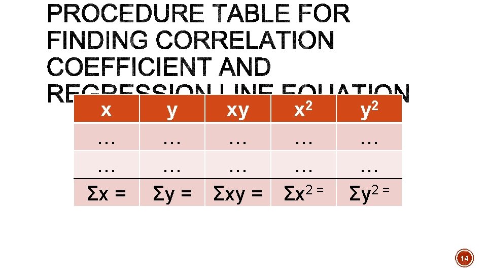
§ where n is the number of data points § round r to 3 decimal places 15

§Compute the correlation coefficient for the data from example 1 and example 2 16

§ Researchers must understand the nature of the linear relationship between the independent variable x and the dependent variable y. When a hypothesis test indicates that a significant linear relationship exists between the variables, researchers must consider the possibilities outlined next… 17

When the null hypothesis has been rejected for a specific alpha value, any of the following five possibilities can exist: 1. There is a direct cause-and-effect relationship between the variables. (x causes y) 2. There is a reverse cause-and-effect relationship between the variables. (y causes x) 3. The relationship between the variables may be caused by a third variable. 4. There may be a complexity of interrelationships among many variables. 5. The relationship may be coincidental. 18

§ When two variables are highly correlated, item 3 in the possible relationships between variables states that there exists a possibility that the correlation is due to a third variable. § If this is the case and the third variable is unknown to the researcher or not accounted for in the study, it is called a lurking variable. § An attempt should be made by the researcher to identify such variables and to use methods to control their influence. § Also , CORRELATION ≠ CAUSATION!!!! 19

§ In studying relationships between two variables, collect the data and then construct a scatter plot. The purpose of the scatter plot, as indicated previously, is to determine the nature of the relationship. The possibilities include: § a positive linear relationship § a negative linear relationship § a curvilinear relationship (won’t talk about) § or no discernible relationship. § The next steps are to compute the correlation coefficient and to test the significance of the relationship. § If the value of the correlation coefficient is significant, the next step is to determine the equation of the regression line, which is the data’s line of best fit. § This allows the researcher to see trends and make predictions about the data. 20

§ Given a scatter plot, you must be able to draw a line of best fit. Best fit means that the sum of the squares of the vertical distances from each point to the line is at a minimum. § The reason you need a line of best fit is that the values of y will be predicted from the values of x; hence, the closer the points are to the line, the better the fit and the prediction will be. § When r is positive, the line slopes upward and to the right. When r is negative, the line slopes downward from left to right. 21

§ a is the y-intercept – round to 3 decimal places § b is the slope of the line – round to 3 decimal places 22

§ Find the equation of the regression line for the data and graph the line on the scatter plot of the data. Company Cars (in thousands) Revenue (in billions) A 63. 0 7. 0 B 29. 0 3. 9 C 20. 8 2. 1 D 19. 1 2. 8 E 13. 4 1. 4 F 8. 5 1. 5 § Use the equation of the regression line to predict the income of a car rental agency that has 200, 000 automobiles. 23

§ Find the equation of the regression line for the data and graph the line on the scatter plot Student Number of Absences Final Grade A 6 82 B 2 86 C 15 43 D 9 74 E 12 58 F 5 90 G 8 78 24

§ The magnitude of the change in one variable when the other variable changes exactly 1 unit is called the marginal change. § Marginal change is represented by b (slope) in your regression equation. § When r is not significantly different from 0, the best predictor of y is the mean of the data values of y. For valid predictions, the value of the correlation coefficient must be significant. § Also two other assumptions must be met… 25

1. For any specific value of the independent variable x, the value of the dependent variable y must be normally distributed about the regression line. 2. The standard deviation of each of the dependent variables must be the same for each value of the independent variable. 26

§ Extrapolation, or making predictions beyond the bounds of the data, must be interpreted cautiously. § When predictions are made, they are based on the present conditions or on the premise that present trends will continue. 27

§ Scatter plots should be checked for outliers. An outlier is a point that seems out of place when compared with the other points. Some of these points can affect the regression line. § When this happens, the points are called influential points or influential observations. Influential points tend to pull the regression line toward itself. § To check for influential points, if a point seems like an outlier, graph the regression line including that points, and then another excluding that point. If the two lines are significantly different, the point can be considered an influential point. § Researchers should use their judgment on whether or not to include an influential point. 28

Total Variation Definition Sum of the squares of the vertical distances each point is from the mean. Divided into explained and unexplained. Equation Equal to the sum of explained and unexplained. Explained Variation Unexplained Variation due to the Variation due to relationship between x chance. and y. When this is small, r Closer r is to +1 or -1, is close to +1 or -1. the better points fir the line and the closer If all points fall on explained variation will regression line, this be to total variation. will be zero. 29

§ Find the three types of variation for the following set of data x 1 2 3 4 5 y 10 8 12 16 20 30

§ The values ( y - y’ ) are called residuals. A residual is the difference between the actual value of y and the predicted value y’ for a given x value. § The mean of the residuals is always zero. § The sum of the squares of the residuals computed by using the regression line is the smallest possible value. For this reason, a regression line is also called a leastsquares line. 31

§ The coefficient of determination is a measure of the variation of the dependent variable that is explained by the regression line and the independent variable. § The coefficient of determination is the ratio of the explained variation to the total variation and is denoted by r 2 = explained variation total variation § r 2 is typically expressed as a percentage of the total variation § Another way to arrive at the coefficient of determination is to square the correlation coefficient 32

§ The rest of the total variation is unexplained, and we call this value the coefficient of nondetermination. § This value is found by subtracting the coefficient of determination from 1. § As the value of r approaches 0, r 2 decreases more rapidly § Coefficient of nondetermination: 1. 00 – r 2 33