Correlation and Linear Regression Chapter 13 13 1

Correlation and Linear Regression Chapter 13 13 -1 Copyright 2018 by Mc. Graw-Hill Education. All rights reserved.

Learning Objectives LO 13 -1 Explain the purpose of correlation analysis LO 13 -2 Calculate a correlation coefficient to test and interpret the relationship between two variables LO 13 -3 Apply regression analysis to estimate the linear relationship between two variables LO 13 -4 Evaluate the significance of the slope of the regression equation LO 13 -5 Evaluate a regression equation’s ability to predict using the standard estimate of the error and the coefficient of determination LO 13 -6 Calculate and interpret confidence and prediction intervals LO 13 -7 Use a log function to transform a nonlinear Copyright 2018 by Mc. Graw-Hill Education. All rights relationship 13 -2 reserved.

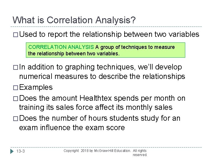
What is Correlation Analysis? � Used to report the relationship between two variables CORRELATION ANALYSIS A group of techniques to measure the relationship between two variables. � In addition to graphing techniques, we’ll develop numerical measures to describe the relationships � Examples � Does the amount Healthtex spends per month on training its sales force affect its monthly sales � Does the number of hours students study for an exam influence the exam score 13 -3 Copyright 2018 by Mc. Graw-Hill Education. All rights reserved.

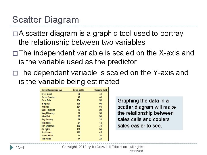
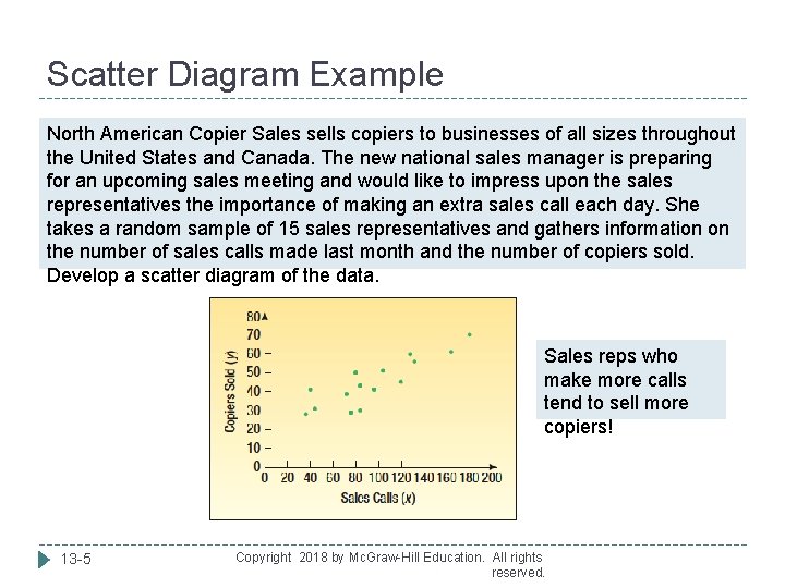
Scatter Diagram � A scatter diagram is a graphic tool used to portray the relationship between two variables � The independent variable is scaled on the X-axis and is the variable used as the predictor � The dependent variable is scaled on the Y-axis and is the variable being estimated Graphing the data in a scatter diagram will make the relationship between sales calls and copiers sales easier to see. 13 -4 Copyright 2018 by Mc. Graw-Hill Education. All rights reserved.

Scatter Diagram Example North American Copier Sales sells copiers to businesses of all sizes throughout the United States and Canada. The new national sales manager is preparing for an upcoming sales meeting and would like to impress upon the sales representatives the importance of making an extra sales call each day. She takes a random sample of 15 sales representatives and gathers information on the number of sales calls made last month and the number of copiers sold. Develop a scatter diagram of the data. Sales reps who make more calls tend to sell more copiers! 13 -5 Copyright 2018 by Mc. Graw-Hill Education. All rights reserved.

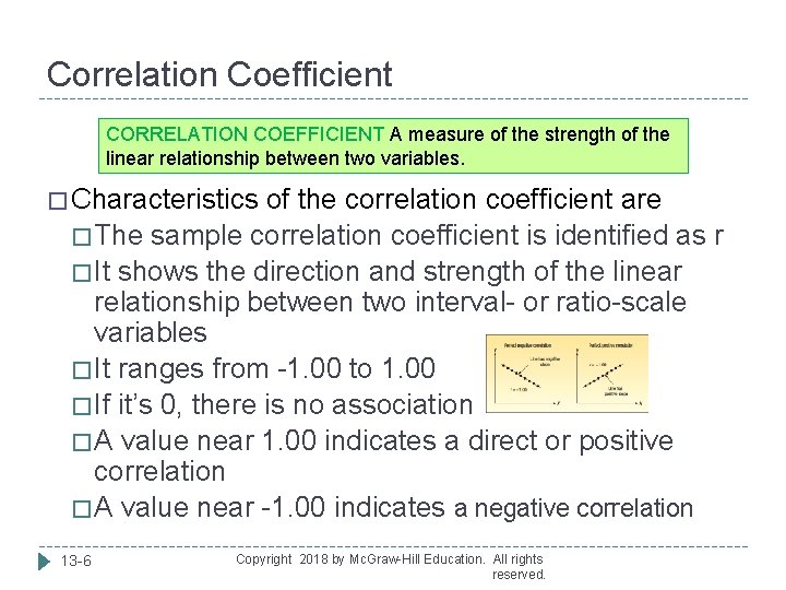
Correlation Coefficient CORRELATION COEFFICIENT A measure of the strength of the linear relationship between two variables. � Characteristics of the correlation coefficient are � The sample correlation coefficient is identified as r � It shows the direction and strength of the linear relationship between two interval- or ratio-scale variables � It ranges from -1. 00 to 1. 00 � If it’s 0, there is no association � A value near 1. 00 indicates a direct or positive correlation � A value near -1. 00 indicates a negative correlation 13 -6 Copyright 2018 by Mc. Graw-Hill Education. All rights reserved.

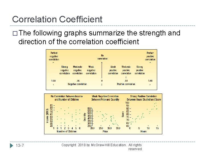
Correlation Coefficient � The following graphs summarize the strength and direction of the correlation coefficient 13 -7 Copyright 2018 by Mc. Graw-Hill Education. All rights reserved.

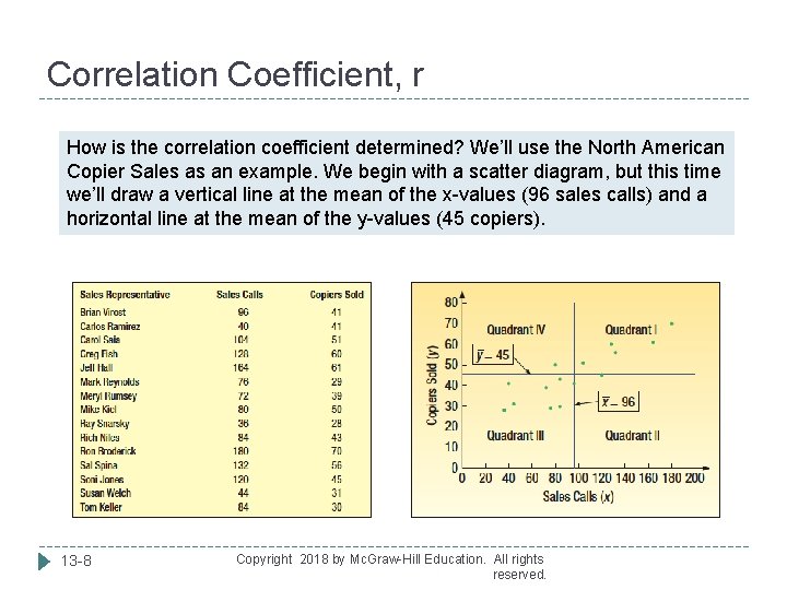
Correlation Coefficient, r How is the correlation coefficient determined? We’ll use the North American Copier Sales as an example. We begin with a scatter diagram, but this time we’ll draw a vertical line at the mean of the x-values (96 sales calls) and a horizontal line at the mean of the y-values (45 copiers). 13 -8 Copyright 2018 by Mc. Graw-Hill Education. All rights reserved.

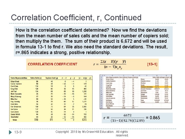
Correlation Coefficient, r, Continued How is the correlation coefficient determined? Now we find the deviations from the mean number of sales calls and the mean number of copiers sold; then multiply them. The sum of their product is 6, 672 and will be used in formula 13 -1 to find r. We also need the standard deviations. The result, r=. 865 indicates a strong, positive relationship. 13 -9 Copyright 2018 by Mc. Graw-Hill Education. All rights reserved.

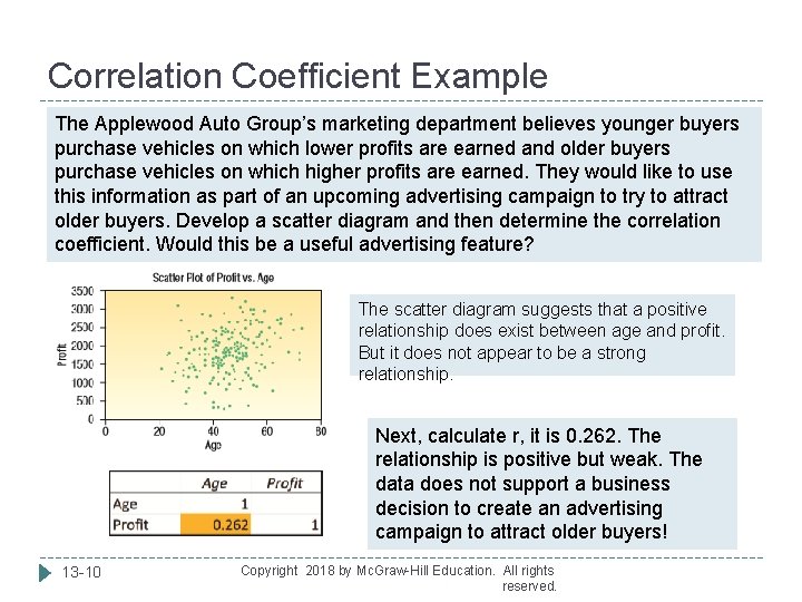
Correlation Coefficient Example The Applewood Auto Group’s marketing department believes younger buyers purchase vehicles on which lower profits are earned and older buyers purchase vehicles on which higher profits are earned. They would like to use this information as part of an upcoming advertising campaign to try to attract older buyers. Develop a scatter diagram and then determine the correlation coefficient. Would this be a useful advertising feature? The scatter diagram suggests that a positive relationship does exist between age and profit. But it does not appear to be a strong relationship. Next, calculate r, it is 0. 262. The relationship is positive but weak. The data does not support a business decision to create an advertising campaign to attract older buyers! 13 -10 Copyright 2018 by Mc. Graw-Hill Education. All rights reserved.

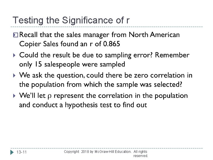
Testing the Significance of r � 13 -11 Copyright 2018 by Mc. Graw-Hill Education. All rights reserved.

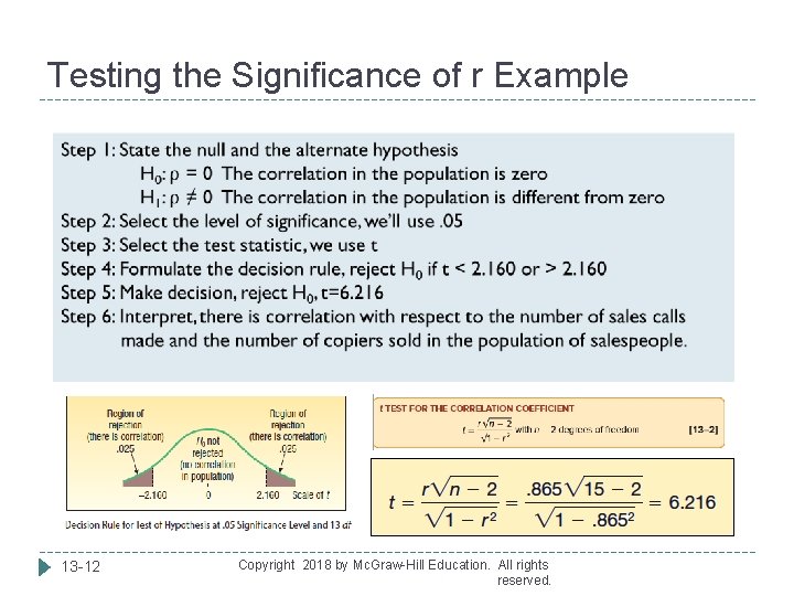
Testing the Significance of r Example 13 -12 Copyright 2018 by Mc. Graw-Hill Education. All rights reserved.

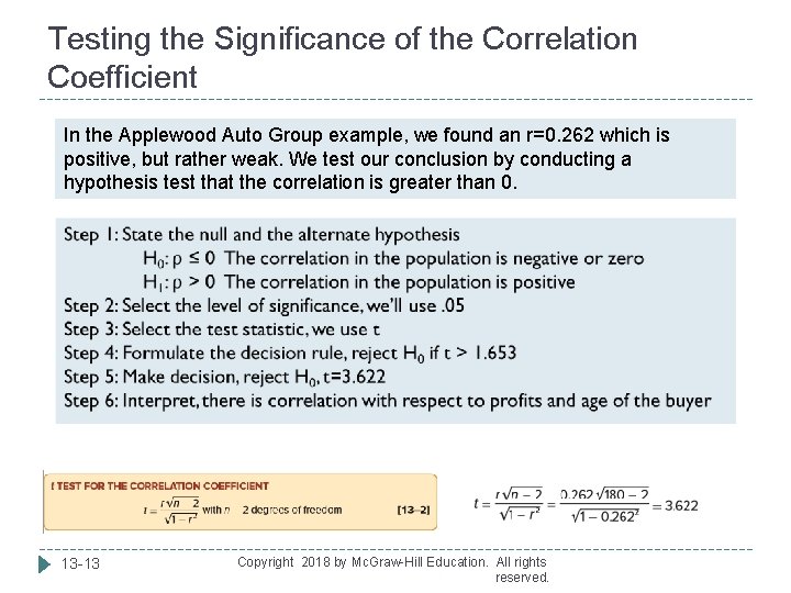
Testing the Significance of the Correlation Coefficient In the Applewood Auto Group example, we found an r=0. 262 which is positive, but rather weak. We test our conclusion by conducting a hypothesis test that the correlation is greater than 0. 13 -13 Copyright 2018 by Mc. Graw-Hill Education. All rights reserved.

Regression Analysis � In regression analysis, we estimate one variable based on another variable � The variable being estimated is the dependent variable � The variable used to make the estimate or predict the value is the independent variable � The relationship between the variables is linear � Both the independent and the dependent variables must be interval or ratio scale REGRESSION EQUATION An equation that expresses the linear relationship between two variables. 13 -14 Copyright 2018 by Mc. Graw-Hill Education. All rights reserved.

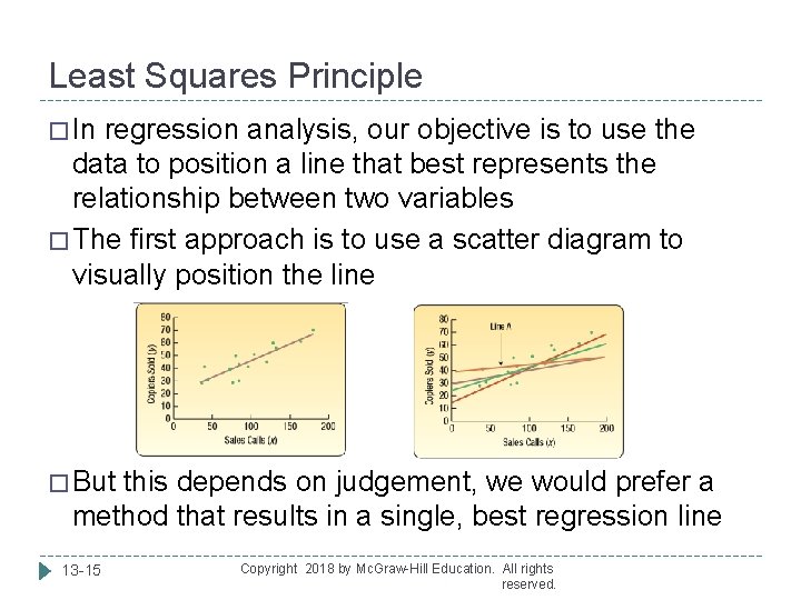
Least Squares Principle � In regression analysis, our objective is to use the data to position a line that best represents the relationship between two variables � The first approach is to use a scatter diagram to visually position the line � But this depends on judgement, we would prefer a method that results in a single, best regression line 13 -15 Copyright 2018 by Mc. Graw-Hill Education. All rights reserved.

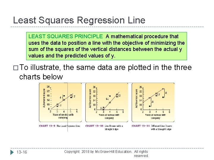
Least Squares Regression Line LEAST SQUARES PRINCIPLE A mathematical procedure that uses the data to position a line with the objective of minimizing the sum of the squares of the vertical distances between the actual y values and the predicted values of y. � To illustrate, the same data are plotted in the three charts below 13 -16 Copyright 2018 by Mc. Graw-Hill Education. All rights reserved.

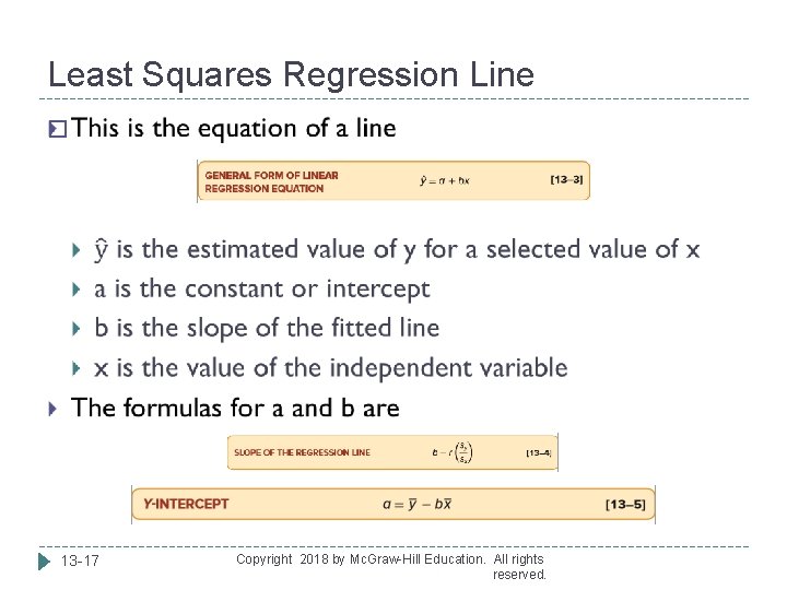
Least Squares Regression Line � 13 -17 Copyright 2018 by Mc. Graw-Hill Education. All rights reserved.

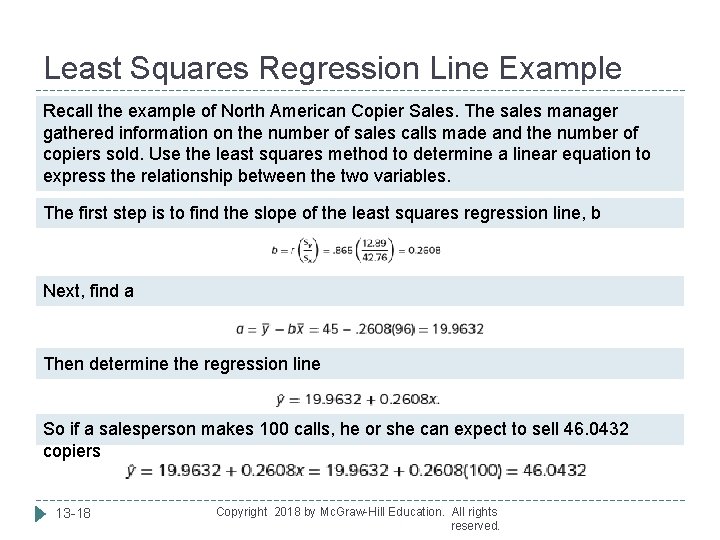
Least Squares Regression Line Example Recall the example of North American Copier Sales. The sales manager gathered information on the number of sales calls made and the number of copiers sold. Use the least squares method to determine a linear equation to express the relationship between the two variables. The first step is to find the slope of the least squares regression line, b Next, find a Then determine the regression line So if a salesperson makes 100 calls, he or she can expect to sell 46. 0432 copiers 13 -18 Copyright 2018 by Mc. Graw-Hill Education. All rights reserved.

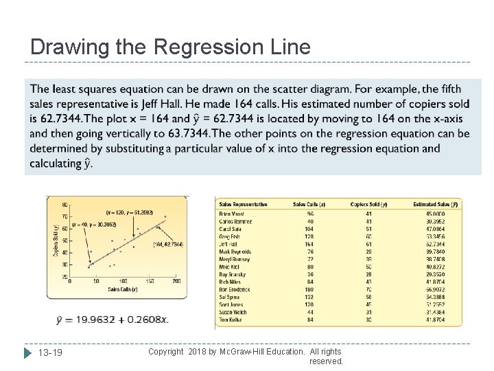
Drawing the Regression Line 13 -19 Copyright 2018 by Mc. Graw-Hill Education. All rights reserved.

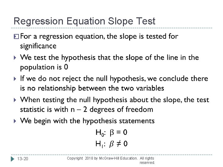
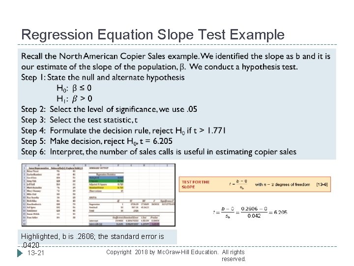
Regression Equation Slope Test � 13 -20 Copyright 2018 by Mc. Graw-Hill Education. All rights reserved.

Regression Equation Slope Test Example Highlighted, b is. 2606; the standard error is . 0420 13 -21 Copyright 2018 by Mc. Graw-Hill Education. All rights reserved.

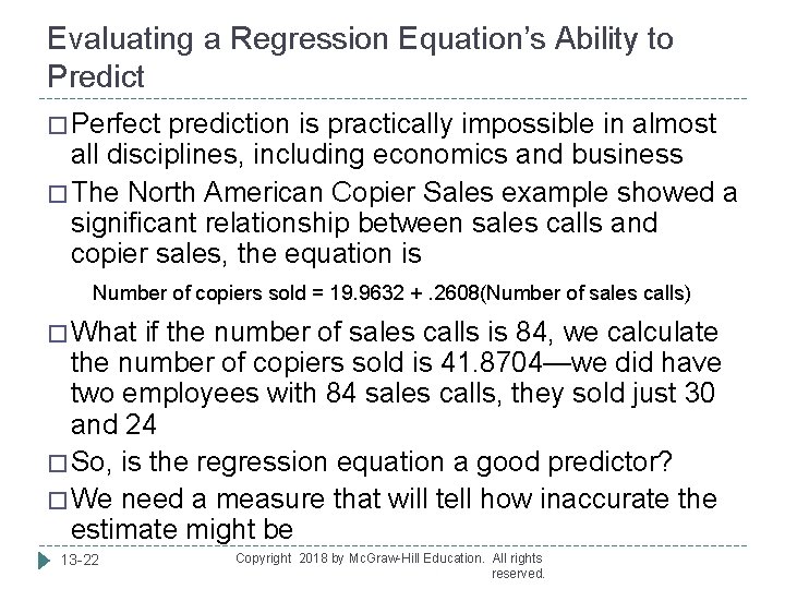
Evaluating a Regression Equation’s Ability to Predict � Perfect prediction is practically impossible in almost all disciplines, including economics and business � The North American Copier Sales example showed a significant relationship between sales calls and copier sales, the equation is Number of copiers sold = 19. 9632 +. 2608(Number of sales calls) � What if the number of sales calls is 84, we calculate the number of copiers sold is 41. 8704—we did have two employees with 84 sales calls, they sold just 30 and 24 � So, is the regression equation a good predictor? � We need a measure that will tell how inaccurate the estimate might be 13 -22 Copyright 2018 by Mc. Graw-Hill Education. All rights reserved.

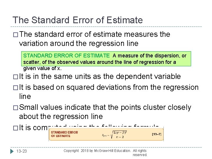
The Standard Error of Estimate � The standard error of estimate measures the variation around the regression line STANDARD ERROR OF ESTIMATE A measure of the dispersion, or scatter, of the observed values around the line of regression for a given value of x. � It is in the same units as the dependent variable � It is based on squared deviations from the regression line � Small values indicate that the points cluster closely about the regression line � It is computed using the following formula 13 -23 Copyright 2018 by Mc. Graw-Hill Education. All rights reserved.

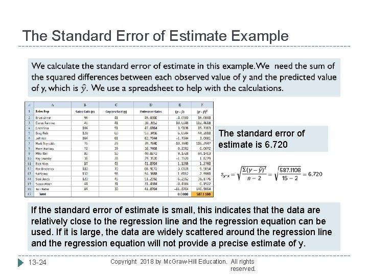
The Standard Error of Estimate Example The standard error of estimate is 6. 720 If the standard error of estimate is small, this indicates that the data are relatively close to the regression line and the regression equation can be used. If it is large, the data are widely scattered around the regression line and the regression equation will not provide a precise estimate of y. 13 -24 Copyright 2018 by Mc. Graw-Hill Education. All rights reserved.

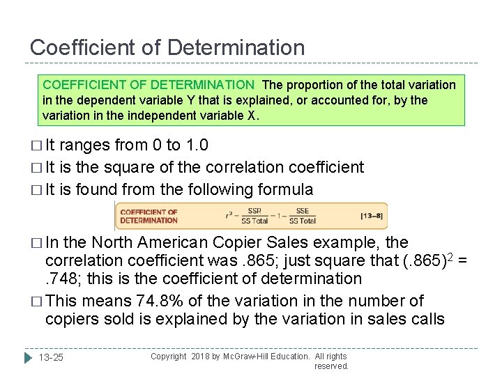
Coefficient of Determination COEFFICIENT OF DETERMINATION The proportion of the total variation in the dependent variable Y that is explained, or accounted for, by the variation in the independent variable X. � It ranges from 0 to 1. 0 � It is the square of the correlation coefficient � It is found from the following formula � In the North American Copier Sales example, the correlation coefficient was. 865; just square that (. 865)2 = . 748; this is the coefficient of determination � This means 74. 8% of the variation in the number of copiers sold is explained by the variation in sales calls 13 -25 Copyright 2018 by Mc. Graw-Hill Education. All rights reserved.

Relationships among r, r 2, and sy, x � Recall the standard error of estimate measures how close the actual values are to the regression line � When it is small, the two variables are closely related � The correlation coefficient measures the strength of the linear association between two variables � When points on the scatter diagram are close to the line, the correlation coefficient tends to be large � Therefore, the correlation coefficient and the standard error of estimate are inversely related � As noted earlier, the coefficient of determination is the correlation coefficient squared 13 -26 Copyright 2018 by Mc. Graw-Hill Education. All rights reserved.

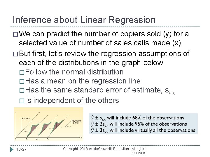
Inference about Linear Regression � We can predict the number of copiers sold (y) for a selected value of number of sales calls made (x) � But first, let’s review the regression assumptions of each of the distributions in the graph below � Follow the normal distribution � Has a mean on the regression line � Has the same standard error of estimate, sy, x � Is independent of the others 13 -27 Copyright 2018 by Mc. Graw-Hill Education. All rights reserved.

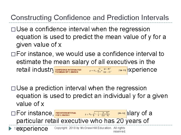
Constructing Confidence and Prediction Intervals � Use a confidence interval when the regression equation is used to predict the mean value of y for a given value of x � For instance, we would use a confidence interval to estimate the mean salary of all executives in the retail industry based on their years of experience � Use a prediction interval when the regression equation is used to predict an individual y for a given value of x � For instance, we would estimate the salary of a particular retail executive who has 20 years of 13 -28 experience Copyright 2018 by Mc. Graw-Hill Education. All rights reserved.

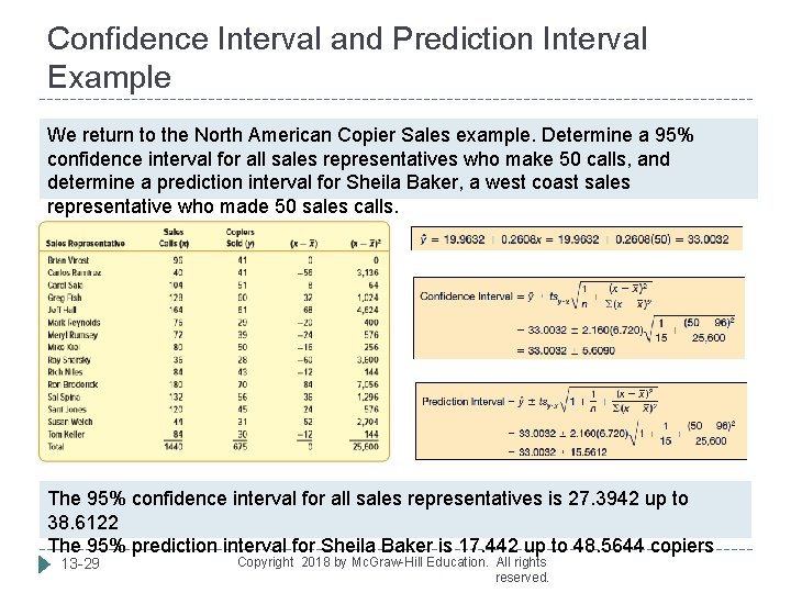
Confidence Interval and Prediction Interval Example We return to the North American Copier Sales example. Determine a 95% confidence interval for all sales representatives who make 50 calls, and determine a prediction interval for Sheila Baker, a west coast sales representative who made 50 sales calls. The 95% confidence interval for all sales representatives is 27. 3942 up to 38. 6122 The 95% prediction interval for Sheila Baker is 17. 442 up to 48. 5644 copiers 13 -29 Copyright 2018 by Mc. Graw-Hill Education. All rights reserved.

Transforming Data � Regression analysis and the correlation coefficient requires data to be linear � But what if data is not linear? � If data is not linear, we can rescale one or both of the variables so the new relationship is linear � Common transformations include � Computing the log to the base 10 of y, Log(y) � Taking the square root � Taking the reciprocal � Squaring one or both variables � Caution: when you are interpreting a correlation coefficient or regression equation – it could be nonlinear Copyright 2018 by Mc. Graw-Hill Education. All rights 13 -30 reserved.

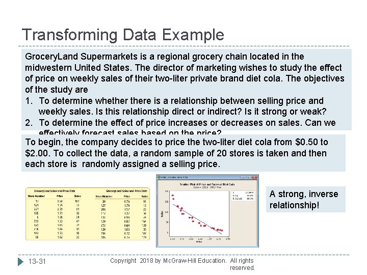
Transforming Data Example Grocery. Land Supermarkets is a regional grocery chain located in the midwestern United States. The director of marketing wishes to study the effect of price on weekly sales of their two-liter private brand diet cola. The objectives of the study are 1. To determine whethere is a relationship between selling price and weekly sales. Is this relationship direct or indirect? Is it strong or weak? 2. To determine the effect of price increases or decreases on sales. Can we effectively forecast sales based on the price? To begin, the company decides to price the two-liter diet cola from $0. 50 to $2. 00. To collect the data, a random sample of 20 stores is taken and then each store is randomly assigned a selling price. A strong, inverse relationship! 13 -31 Copyright 2018 by Mc. Graw-Hill Education. All rights reserved.

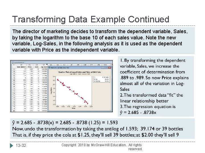
Transforming Data Example Continued The director of marketing decides to transform the dependent variable, Sales, by taking the logarithm to the base 10 of each sales value. Note the new variable, Log-Sales, in the following analysis as it is used as the dependent variable with Price as the independent variable. 13 -32 Copyright 2018 by Mc. Graw-Hill Education. All rights reserved.