Correlation Analysis Copyright c 2008 by The Mc

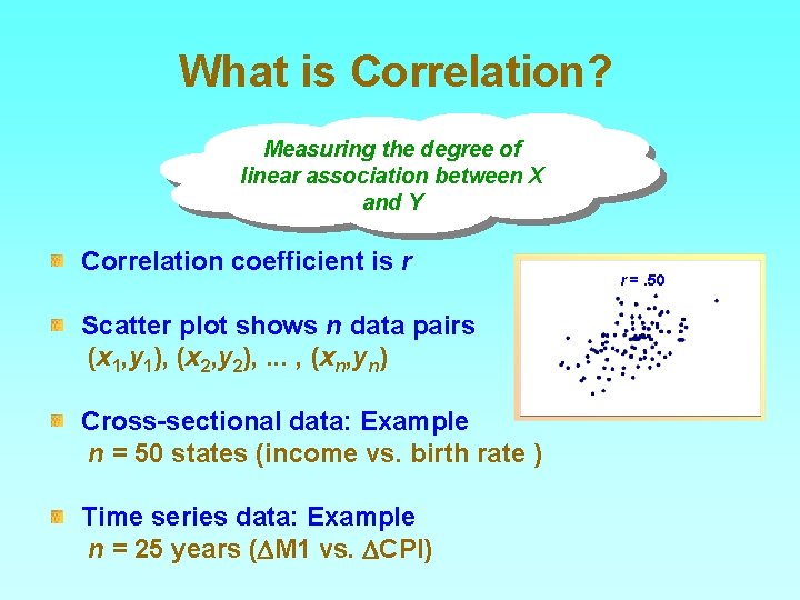
What is Correlation? Measuring the degree of linear association between X and Y What Is Correlation? Correlation coefficient is r Scatter plot shows n data pairs (x 1, y 1), (x 2, y 2), . . . , (xn, yn) Cross-sectional data: Example n = 50 states (income vs. birth rate ) Time series data: Example n = 25 years (DM 1 vs. DCPI) r =. 50

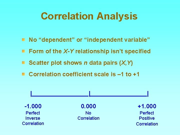
Correlation Analysis No “dependent” or “independent variable” Form of the X-Y relationship isn’t specified Scatter plot shows n data pairs (X, Y) Correlation coefficient scale is – 1 to +1 |_________________| -1. 000 0. 000 +1. 000 Perfect Inverse Correlation No Correlation Perfect Positive Correlation

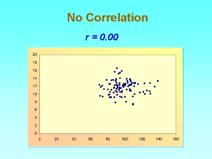
No Correlation r = 0. 00

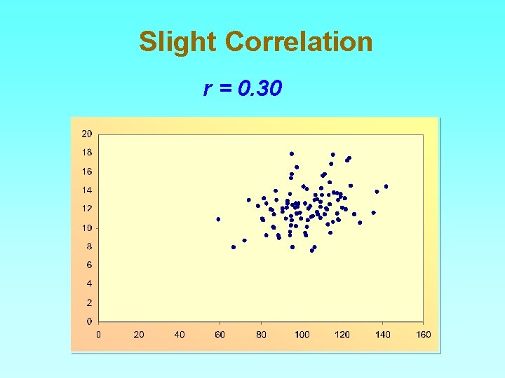
Slight Correlation r = 0. 30

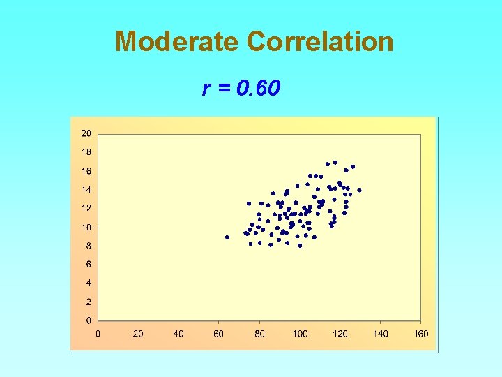
Moderate Correlation r = 0. 60

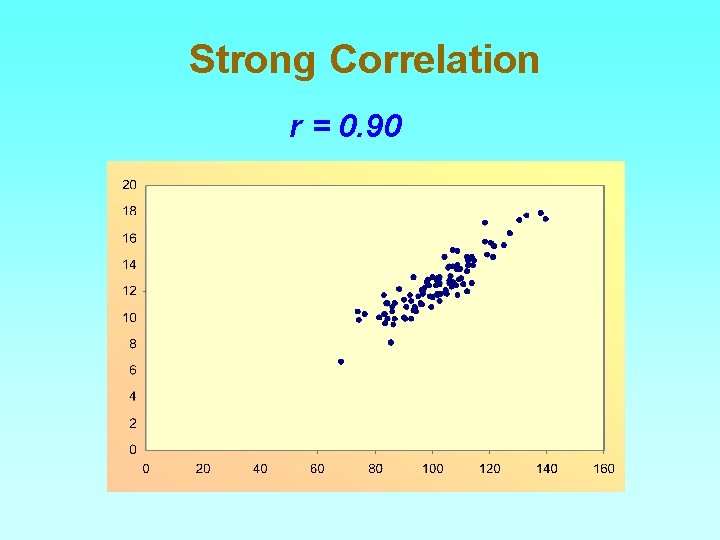
Strong Correlation r = 0. 90

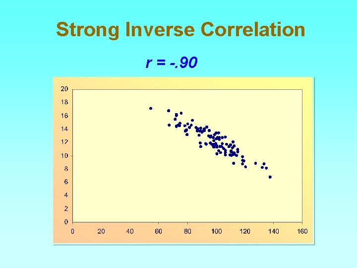
Strong Inverse Correlation r = -. 90

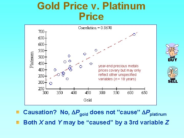
Gold Price v. Platinum Price year-end precious metals prices covary but may only reflect other unspecified variables (n = 18 years) Causation? No, DPgold does not "cause" DPplatinum Both X and Y may be “caused” by a 3 rd variable Z

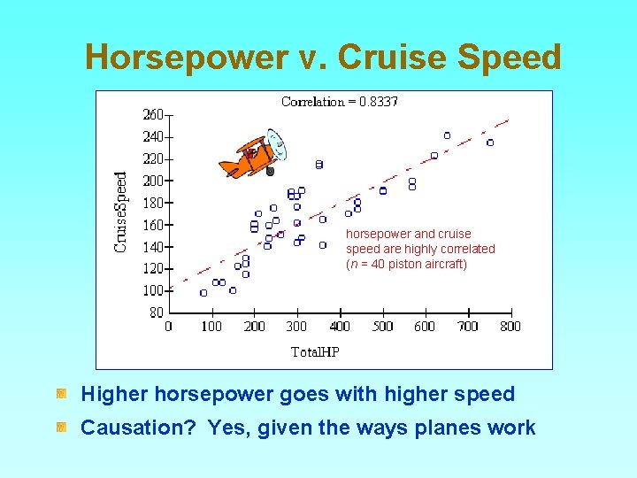
Horsepower v. Cruise Speed horsepower and cruise speed are highly correlated (n = 40 piston aircraft) Higher horsepower goes with higher speed Causation? Yes, given the ways planes work

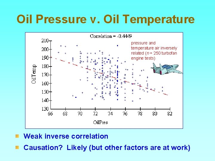
Oil Pressure v. Oil Temperature pressure and temperature air inversely related (n = 250 turbofan engine tests) Weak inverse correlation Causation? Likely (but other factors are at work)

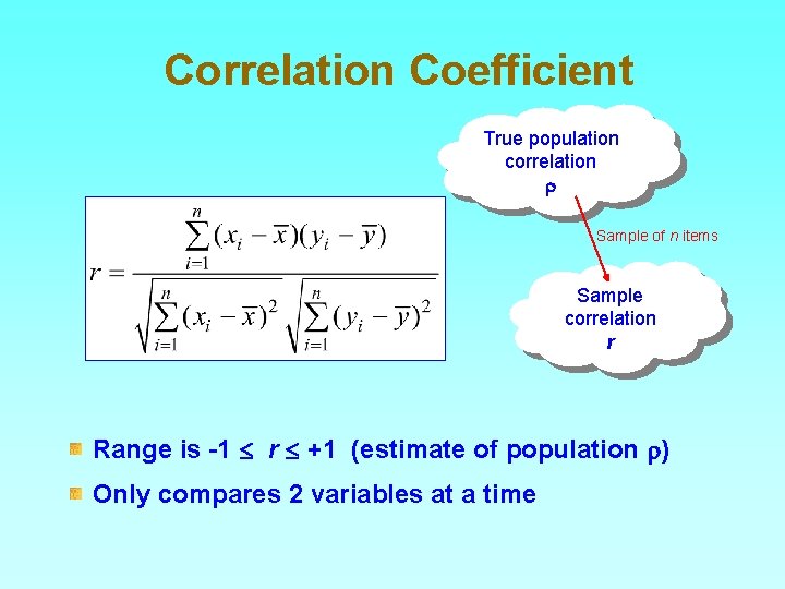
Correlation Coefficient True population correlation r Sample of n items Sample correlation r Range is -1 r +1 (estimate of population r) Only compares 2 variables at a time

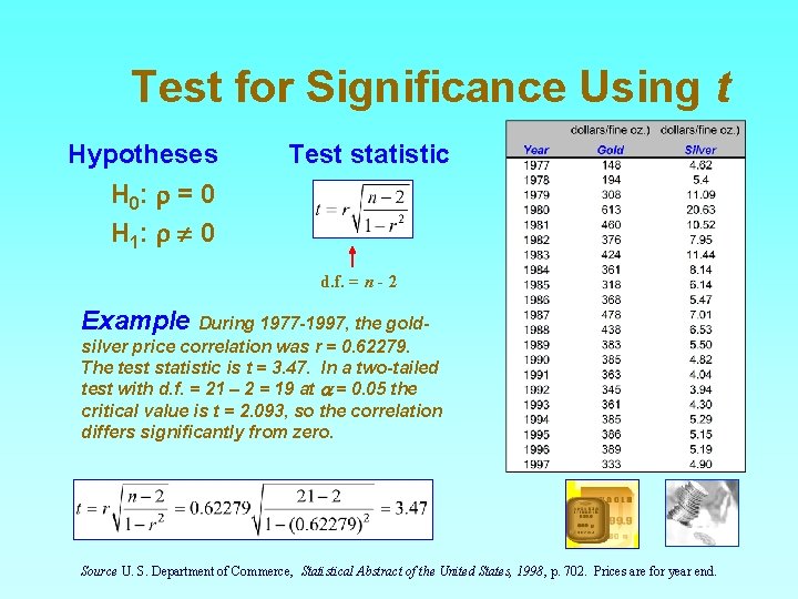
Test for Significance Using t Hypotheses Test statistic H 0: r = 0 H 1: r 0 d. f. = n - 2 Example During 1977 -1997, the goldsilver price correlation was r = 0. 62279. The test statistic is t = 3. 47. In a two-tailed test with d. f. = 21 – 2 = 19 at a = 0. 05 the critical value is t = 2. 093, so the correlation differs significantly from zero. Source U. S. Department of Commerce, Statistical Abstract of the United States, 1998, p. 702. Prices are for year end.

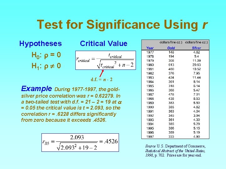
Test for Significance Using r Hypotheses Critical Value H 0: r = 0 H 1: r 0 d. f. = n - 2 Example During 1977 -1997, the goldsilver price correlation was r = 0. 62279. In a two-tailed test with d. f. = 21 – 2 = 19 at a = 0. 05 the critical value is t = 2. 093, so the correlation r =. 6228 differs significantly from zero because it exceeds. 4526. Source U. S. Department of Commerce, Statistical Abstract of the United States, 1998, p. 702. Prices are for year end.

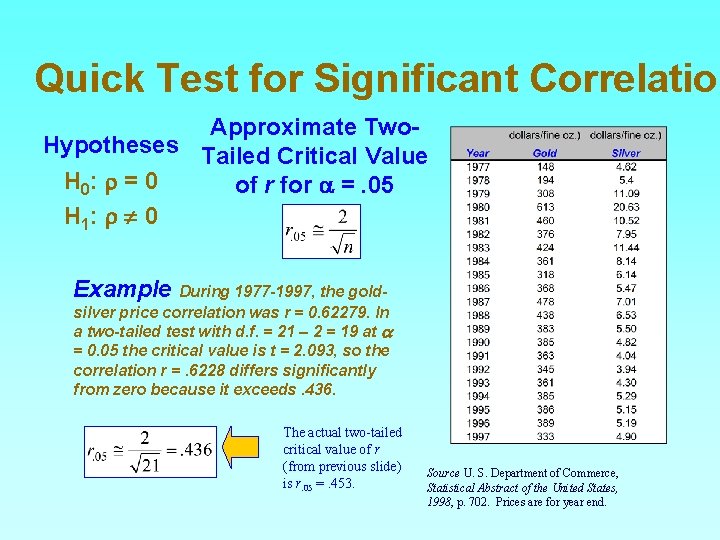
Quick Test for Significant Correlation Approximate Two. Hypotheses Tailed Critical Value H 0: r = 0 of r for a =. 05 H 1: r 0 Example During 1977 -1997, the goldsilver price correlation was r = 0. 62279. In a two-tailed test with d. f. = 21 – 2 = 19 at a = 0. 05 the critical value is t = 2. 093, so the correlation r =. 6228 differs significantly from zero because it exceeds. 436. The actual two-tailed critical value of r (from previous slide) is r. 05 =. 453. Source U. S. Department of Commerce, Statistical Abstract of the United States, 1998, p. 702. Prices are for year end.

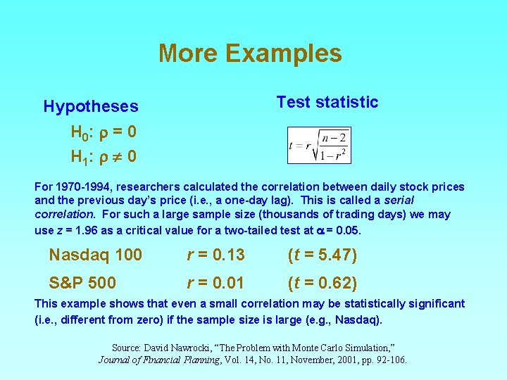
More Examples Test statistic Hypotheses H 0: r = 0 H 1: r 0 For 1970 -1994, researchers calculated the correlation between daily stock prices and the previous day’s price (i. e. , a one-day lag). This is called a serial correlation. For such a large sample size (thousands of trading days) we may use z = 1. 96 as a critical value for a two-tailed test at a = 0. 05. Nasdaq 100 r = 0. 13 (t = 5. 47) S&P 500 r = 0. 01 (t = 0. 62) This example shows that even a small correlation may be statistically significant (i. e. , different from zero) if the sample size is large (e. g. , Nasdaq). Source: David Nawrocki, “The Problem with Monte Carlo Simulation, ” Journal of Financial Planning, Vol. 14, No. 11, November, 2001, pp. 92 -106.

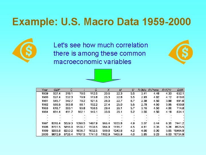
Example: U. S. Macro Data 1959 -2000 Let's see how much correlation there is among these common macroeconomic variables

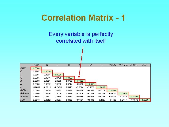
Correlation Matrix - 1 Every variable is perfectly correlated with itself

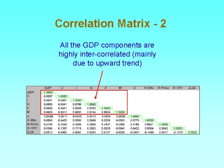
Correlation Matrix - 2 All the GDP components are highly inter-correlated (mainly due to upward trend)

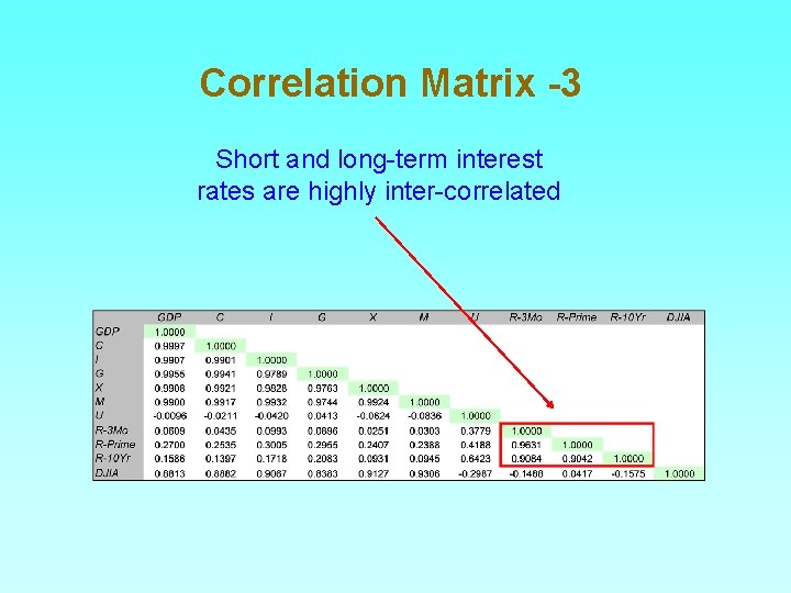
Correlation Matrix -3 Short and long-term interest rates are highly inter-correlated

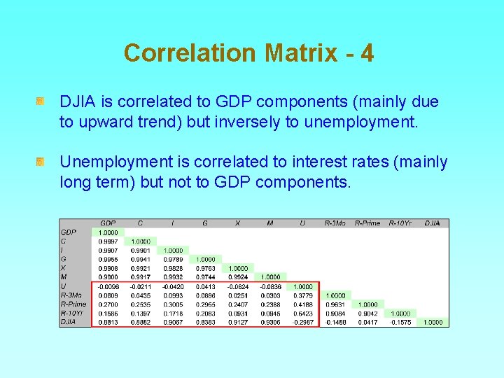
Correlation Matrix - 4 DJIA is correlated to GDP components (mainly due to upward trend) but inversely to unemployment. Unemployment is correlated to interest rates (mainly long term) but not to GDP components.

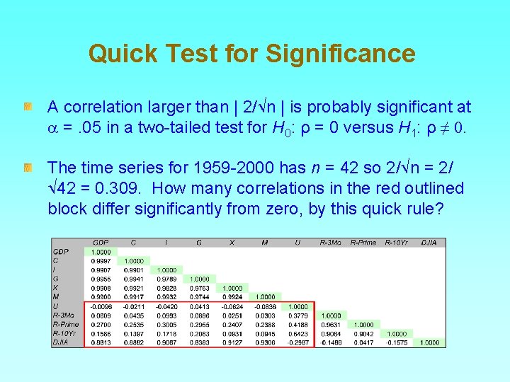
Quick Test for Significance A correlation larger than | 2/ n | is probably significant at =. 05 in a two-tailed test for H 0: ρ = 0 versus H 1: ρ ≠ 0. The time series for 1959 -2000 has n = 42 so 2/ n = 2/ 42 = 0. 309. How many correlations in the red outlined block differ significantly from zero, by this quick rule?

Limitations It's easy to find X-Y correlations They show linear X-Y association They don't prove X is a cause of Y Multiple causes are likely Bottom Line If you want to explain something, you need to go beyond simple correlations.