Copyright The Mc GrawHill Companies Inc Permission required

Section 3. 3 - Objectives 1. 2. 3. 4. 5. 6. Compute and interpret

Objective 1 Compute and interpret z-scores Copyright © The Mc. Graw-Hill Companies, Inc. Permission

z-Score Who is taller, a man 73 inches tall or a woman 68 inches

z-Score The z-score of an individual data value tells how many standard deviations that

Example 3. 22 A National Center for Health Statistics study states that the mean

Solution We compute the z-scores for the two heights. Taller, relative to the population

z-Scores & The Empirical Rule Since the z-score is the number of standard deviations

Objective 2 Compute percentiles of a data set Copyright © The Mc. Graw-Hill Companies,

Objective 3 Compute the quartiles of a data set Copyright © The Mc. Graw-Hill

Quartiles There are three special percentiles which divide a data set into four pieces,

Example 3. 25 The following table presents the annual rainfall, in inches, in Los

Solution Step 1: Arrange the data in increasing order. 0. 00 1. 48 4.

Quartiles on the TI-84 PLUS On the TI-84 PLUS Calculator, the 1 -Var Stats

Objective 4 Compute the five-number summary for a data set Copyright © The Mc.

Five-Number Summary The five-number summary of a data set consists of the median, the

Example – Five-Number Summary Consider again the Los Angeles rainfall data. 0. 00 1.

Objective 5 Understand the effects of outliers Copyright © The Mc. Graw-Hill Companies, Inc.

Outliers An outlier is a value that is considerably larger or considerably smaller than

Example 3. 28 The temperature in a downtown location in a certain city is

Interquartile Range One method for detecting outliers involves a measure called the Interquartile Range.

IQR Method for Detecting Outliers The most frequent method used to detect outliers in

Example 3. 30 The following table presents the number of students absent in a

Solution We may use the TI-84 PLUS, or other technology, to compute the quartiles.

Solution The Interquartile Range is IQR = Q 3 – Q 1 = 59

Objective 6 Construct boxplots to visualize the fivenumber summary and outliers Copyright © The

Any Data Set A boxplot is a graph that presents the five-number summary along

Procedure for Drawing a Boxplot Following is the procedure for drawing a boxplot: Step

Example 3. 31 The following table presents the number of students absent in a

Solution Step 1: We may use the TI-84 PLUS, or other technology, to compute

Solution Step 2: We draw vertical lines at 45, 51, and 59, then horizontal

Solution Step 4: The largest data value that is less than the upper boundary

Solution Step 5: The smallest data value that is greater than the lower boundary

Solution Step 6: The data value 100 lies outside of the outlier boundaries. Therefore,

Determining Skewness Boxplots can help determine the skewness of a data set. If the

Determining Skewness If the median is closer to the third quartile than to the

Determining Skewness If the median is approximately halfway between the first and third quartiles,

Do You Know… • • • How to compute and interpret z-scores? How to

Slides: 38

Download presentation

Section 3. 3 - Objectives 1. 2. 3. 4. 5. 6. Compute and interpret z-scores Compute percentiles of a data set Compute the quartiles of a data set Compute the five-number summary for a data set Understand the effects of outliers Construct boxplots to visualize the five-number summary and outliers Copyright © The Mc. Graw-Hill Companies, Inc. Permission required for reproduction or display.

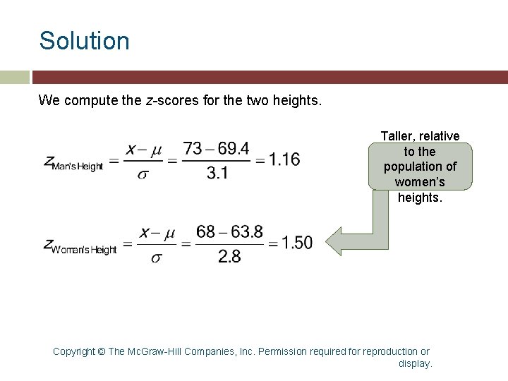
z-Score Who is taller, a man 73 inches tall or a woman 68 inches tall? The obvious answer is that the man is taller. However, men are taller than women on the average. Suppose the question is asked this way: Who is taller relative to their gender, a man 73 inches tall or a woman 68 inches tall? One way to answer this question is with a z-score. Copyright © The Mc. Graw-Hill Companies, Inc. Permission required for reproduction or display.

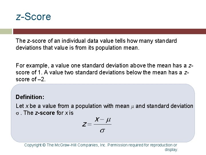
z-Score The z-score of an individual data value tells how many standard deviations that value is from its population mean. For example, a value one standard deviation above the mean has a zscore of 1. A value two standard deviations below the mean has a zscore of – 2. Definition: Let x be a value from a population with mean μ and standard deviation σ. The z-score for x is Copyright © The Mc. Graw-Hill Companies, Inc. Permission required for reproduction or display.

Example 3. 22 A National Center for Health Statistics study states that the mean height for adult men in the U. S. is μ = 69. 4 inches, with a standard deviation of σ = 3. 1 inches. The mean height for adult women is μ = 63. 8 inches, with a standard deviation of σ = 2. 8 inches. Who is taller relative to their gender, a man 73 inches tall, or a woman 68 inches tall? Copyright © The Mc. Graw-Hill Companies, Inc. Permission required for reproduction or display.

Solution We compute the z-scores for the two heights. Taller, relative to the population of women’s heights. Copyright © The Mc. Graw-Hill Companies, Inc. Permission required for reproduction or display.

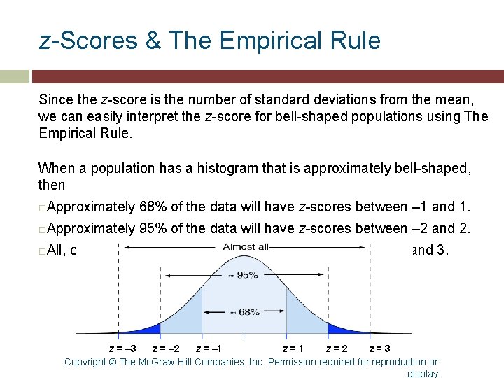
z-Scores & The Empirical Rule Since the z-score is the number of standard deviations from the mean, we can easily interpret the z-score for bell-shaped populations using The Empirical Rule. When a population has a histogram that is approximately bell-shaped, then Approximately 68% of the data will have z-scores between – 1 and 1. Approximately 95% of the data will have z-scores between – 2 and 2. All, or almost all of the data will have z-scores between – 3 and 3. z = – 3 z = – 2 z = – 1 z=2 z=3 Copyright © The Mc. Graw-Hill Companies, Inc. Permission required for reproduction or display.

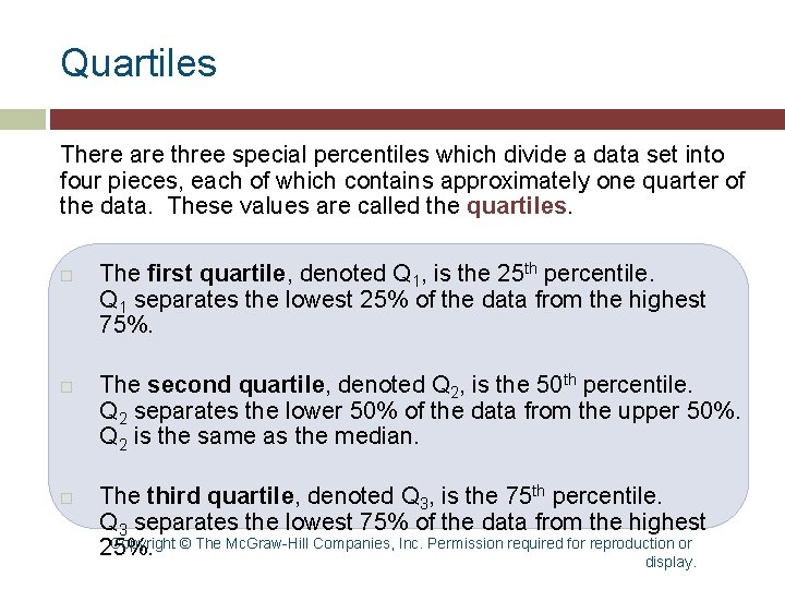
Quartiles There are three special percentiles which divide a data set into four pieces, each of which contains approximately one quarter of the data. These values are called the quartiles. The first quartile, denoted Q 1, is the 25 th percentile. Q 1 separates the lowest 25% of the data from the highest 75%. The second quartile, denoted Q 2, is the 50 th percentile. Q 2 separates the lower 50% of the data from the upper 50%. Q 2 is the same as the median. The third quartile, denoted Q 3, is the 75 th percentile. Q 3 separates the lowest 75% of the data from the highest Copyright © The Mc. Graw-Hill Companies, Inc. Permission required for reproduction or 25%. display.

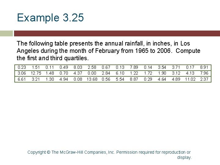
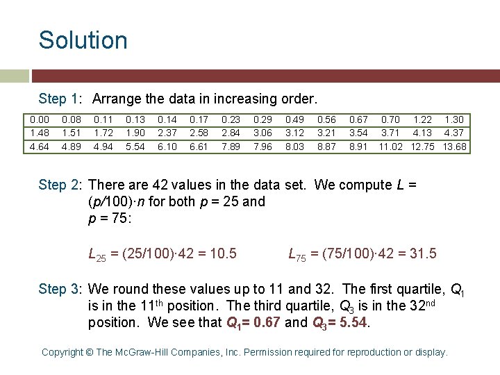
Example 3. 25 The following table presents the annual rainfall, in inches, in Los Angeles during the month of February from 1965 to 2006. Compute the first and third quartiles. 0. 23 3. 06 6. 61 1. 51 12. 75 3. 21 0. 11 1. 48 1. 30 0. 49 0. 70 4. 94 8. 03 4. 37 0. 08 2. 58 0. 00 13. 68 0. 67 2. 84 0. 56 0. 13 6. 10 5. 54 7. 89 1. 22 8. 87 0. 14 1. 72 0. 29 3. 54 1. 90 4. 64 3. 71 3. 12 4. 89 0. 17 4. 13 11. 02 Copyright © The Mc. Graw-Hill Companies, Inc. Permission required for reproduction or display. 8. 91 7. 96 2. 37

Solution Step 1: Arrange the data in increasing order. 0. 00 1. 48 4. 64 0. 08 1. 51 4. 89 0. 11 1. 72 4. 94 0. 13 1. 90 5. 54 0. 14 2. 37 6. 10 0. 17 2. 58 6. 61 0. 23 2. 84 7. 89 0. 29 3. 06 7. 96 0. 49 3. 12 8. 03 0. 56 3. 21 8. 87 0. 67 3. 54 8. 91 0. 70 1. 22 1. 30 3. 71 4. 13 4. 37 11. 02 12. 75 13. 68 Step 2: There are 42 values in the data set. We compute L = (p/100)·n for both p = 25 and p = 75: L 25 = (25/100)· 42 = 10. 5 L 75 = (75/100)· 42 = 31. 5 Step 3: We round these values up to 11 and 32. The first quartile, Q 1 is in the 11 th position. The third quartile, Q 3 is in the 32 nd position. We see that Q 1= 0. 67 and Q 3= 5. 54. Copyright © The Mc. Graw-Hill Companies, Inc. Permission required for reproduction or display.

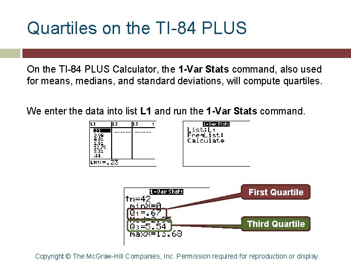
Quartiles on the TI-84 PLUS On the TI-84 PLUS Calculator, the 1 -Var Stats command, also used for means, medians, and standard deviations, will compute quartiles. We enter the data into list L 1 and run the 1 -Var Stats command. First Quartile Third Quartile Copyright © The Mc. Graw-Hill Companies, Inc. Permission required for reproduction or display.

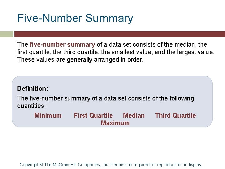
Five-Number Summary The five-number summary of a data set consists of the median, the first quartile, the third quartile, the smallest value, and the largest value. These values are generally arranged in order. Definition: The five-number summary of a data set consists of the following quantities: Minimum First Quartile Median Maximum Third Quartile Copyright © The Mc. Graw-Hill Companies, Inc. Permission required for reproduction or display.

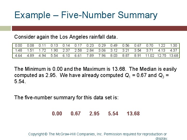
Example – Five-Number Summary Consider again the Los Angeles rainfall data. 0. 00 1. 48 4. 64 0. 08 1. 51 4. 89 0. 11 1. 72 4. 94 0. 13 1. 90 5. 54 0. 14 2. 37 6. 10 0. 17 2. 58 6. 61 0. 23 2. 84 7. 89 0. 29 3. 06 7. 96 0. 49 3. 12 8. 03 0. 56 3. 21 8. 87 0. 67 3. 54 8. 91 0. 70 1. 22 1. 30 3. 71 4. 13 4. 37 11. 02 12. 75 13. 68 The Minimum is 0. 00 and the Maximum is 13. 68. The Median is easily computed as 2. 95. We have already computed Q 1 = 0. 67 and Q 3 = 5. 54. The five-number summary for this data set is: 0. 00 0. 67 2. 95 5. 54 13. 68 Copyright © The Mc. Graw-Hill Companies, Inc. Permission required for reproduction or display.

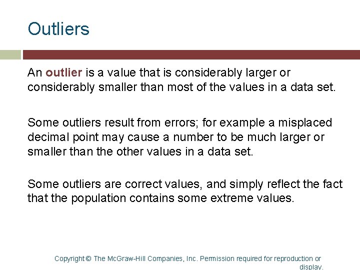
Outliers An outlier is a value that is considerably larger or considerably smaller than most of the values in a data set. Some outliers result from errors; for example a misplaced decimal point may cause a number to be much larger or smaller than the other values in a data set. Some outliers are correct values, and simply reflect the fact that the population contains some extreme values. Copyright © The Mc. Graw-Hill Companies, Inc. Permission required for reproduction or display.

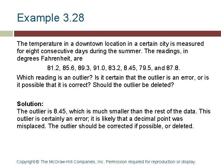
Example 3. 28 The temperature in a downtown location in a certain city is measured for eight consecutive days during the summer. The readings, in degrees Fahrenheit, are 81. 2, 85. 6, 89. 3, 91. 0, 83. 2, 8. 45, 79. 5, and 87. 8. Which reading is an outlier? Is it certain that the outlier is an error, or is it possible that it is correct? Should the outlier be deleted? Solution: The outlier is 8. 45, which is much smaller than the rest of the data. This outlier is certainly an error; it is likely that a decimal point was misplaced. The outlier should be corrected if possible, or deleted. Copyright © The Mc. Graw-Hill Companies, Inc. Permission required for reproduction or display.

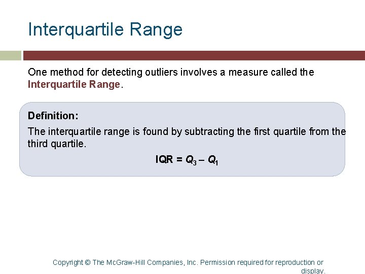
Interquartile Range One method for detecting outliers involves a measure called the Interquartile Range. Definition: The interquartile range is found by subtracting the first quartile from the third quartile. IQR = Q 3 – Q 1 Copyright © The Mc. Graw-Hill Companies, Inc. Permission required for reproduction or display.

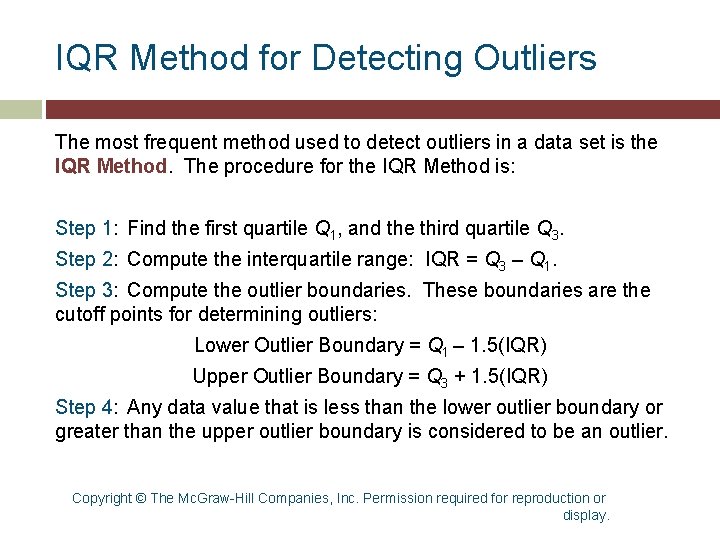
IQR Method for Detecting Outliers The most frequent method used to detect outliers in a data set is the IQR Method. The procedure for the IQR Method is: Step 1: Find the first quartile Q 1, and the third quartile Q 3. Step 2: Compute the interquartile range: IQR = Q 3 – Q 1. Step 3: Compute the outlier boundaries. These boundaries are the cutoff points for determining outliers: Lower Outlier Boundary = Q 1 – 1. 5(IQR) Upper Outlier Boundary = Q 3 + 1. 5(IQR) Step 4: Any data value that is less than the lower outlier boundary or greater than the upper outlier boundary is considered to be an outlier. Copyright © The Mc. Graw-Hill Companies, Inc. Permission required for reproduction or display.

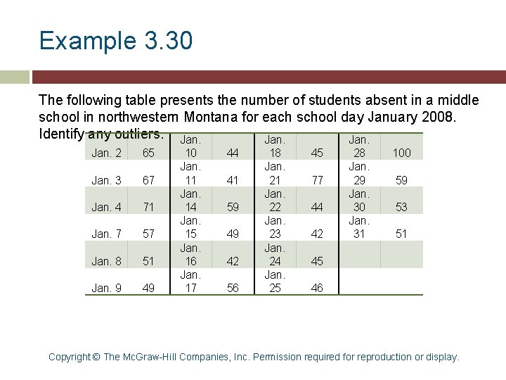
Example 3. 30 The following table presents the number of students absent in a middle school in northwestern Montana for each school day January 2008. Identify any outliers. Jan. 2 65 Jan. 3 67 Jan. 4 71 Jan. 7 57 Jan. 8 51 Jan. 9 49 10 Jan. 11 Jan. 14 Jan. 15 Jan. 16 Jan. 17 44 41 59 49 42 56 18 Jan. 21 Jan. 22 Jan. 23 Jan. 24 Jan. 25 45 77 44 42 28 Jan. 29 Jan. 30 Jan. 31 100 59 53 51 45 46 Copyright © The Mc. Graw-Hill Companies, Inc. Permission required for reproduction or display.

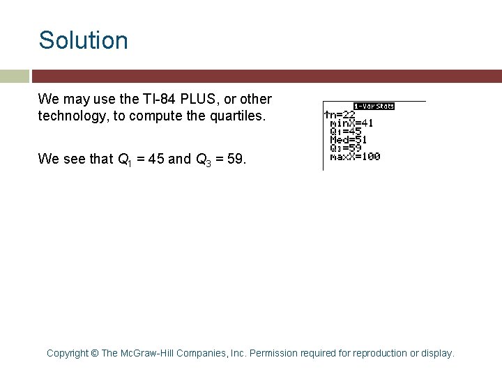
Solution We may use the TI-84 PLUS, or other technology, to compute the quartiles. We see that Q 1 = 45 and Q 3 = 59. Copyright © The Mc. Graw-Hill Companies, Inc. Permission required for reproduction or display.

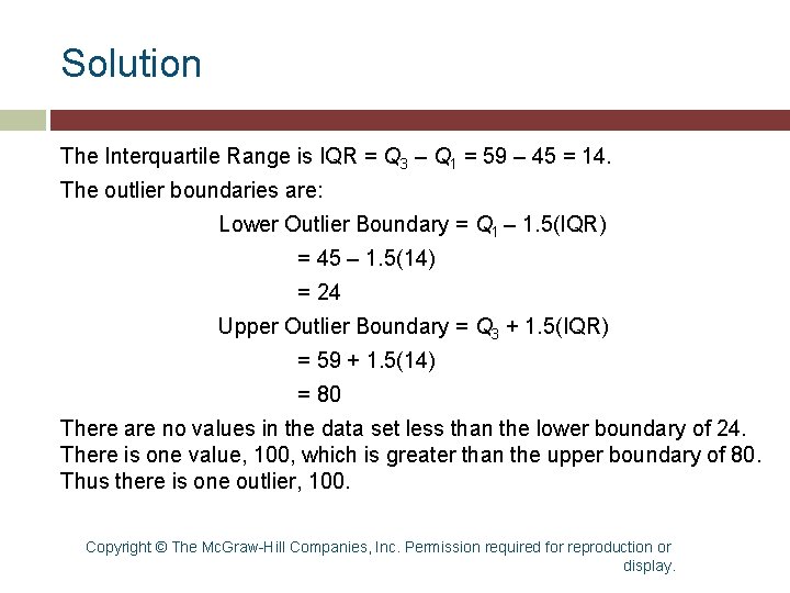
Solution The Interquartile Range is IQR = Q 3 – Q 1 = 59 – 45 = 14. The outlier boundaries are: Lower Outlier Boundary = Q 1 – 1. 5(IQR) = 45 – 1. 5(14) = 24 Upper Outlier Boundary = Q 3 + 1. 5(IQR) = 59 + 1. 5(14) = 80 There are no values in the data set less than the lower boundary of 24. There is one value, 100, which is greater than the upper boundary of 80. Thus there is one outlier, 100. Copyright © The Mc. Graw-Hill Companies, Inc. Permission required for reproduction or display.

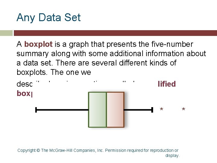
Any Data Set A boxplot is a graph that presents the five-number summary along with some additional information about a data set. There are several different kinds of boxplots. The one we describe here is sometimes called a modified boxplot. * Copyright © The Mc. Graw-Hill Companies, Inc. Permission required for reproduction or display. *

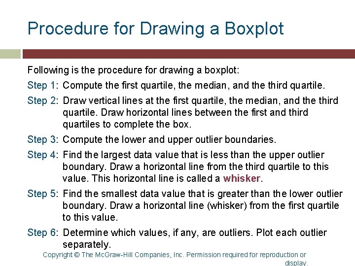
Procedure for Drawing a Boxplot Following is the procedure for drawing a boxplot: Step 1: Compute the first quartile, the median, and the third quartile. Step 2: Draw vertical lines at the first quartile, the median, and the third quartile. Draw horizontal lines between the first and third quartiles to complete the box. Step 3: Compute the lower and upper outlier boundaries. Step 4: Find the largest data value that is less than the upper outlier boundary. Draw a horizontal line from the third quartile to this value. This horizontal line is called a whisker. Step 5: Find the smallest data value that is greater than the lower outlier boundary. Draw a horizontal line (whisker) from the first quartile to this value. Step 6: Determine which values, if any, are outliers. Plot each outlier separately. Copyright © The Mc. Graw-Hill Companies, Inc. Permission required for reproduction or display.

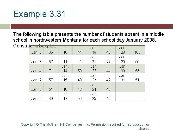
Example 3. 31 The following table presents the number of students absent in a middle school in northwestern Montana for each school day January 2008. Construct a boxplot. Jan. 2 65 Jan. 3 67 Jan. 4 71 Jan. 7 57 Jan. 8 51 Jan. 9 49 10 Jan. 11 Jan. 14 Jan. 15 Jan. 16 Jan. 17 44 41 59 49 42 56 18 Jan. 21 Jan. 22 Jan. 23 Jan. 24 Jan. 25 45 77 44 42 28 Jan. 29 Jan. 30 Jan. 31 100 59 53 51 45 46 Copyright © The Mc. Graw-Hill Companies, Inc. Permission required for reproduction or display.

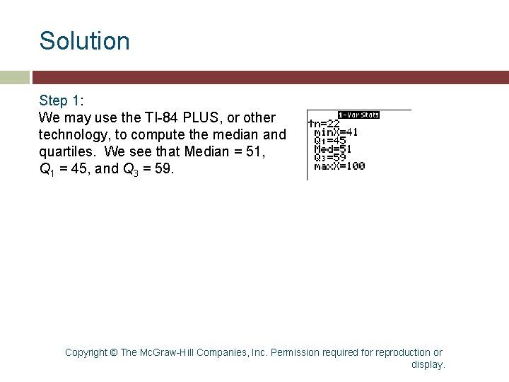
Solution Step 1: We may use the TI-84 PLUS, or other technology, to compute the median and quartiles. We see that Median = 51, Q 1 = 45, and Q 3 = 59. Copyright © The Mc. Graw-Hill Companies, Inc. Permission required for reproduction or display.

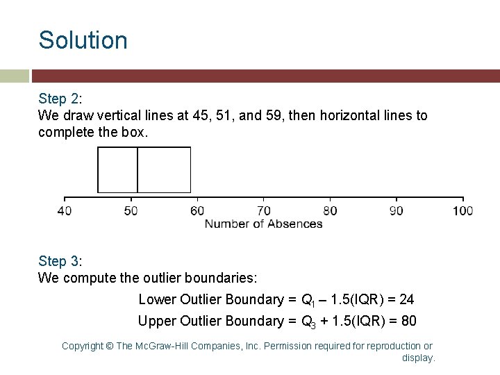
Solution Step 2: We draw vertical lines at 45, 51, and 59, then horizontal lines to complete the box. Step 3: We compute the outlier boundaries: Lower Outlier Boundary = Q 1 – 1. 5(IQR) = 24 Upper Outlier Boundary = Q 3 + 1. 5(IQR) = 80 Copyright © The Mc. Graw-Hill Companies, Inc. Permission required for reproduction or display.

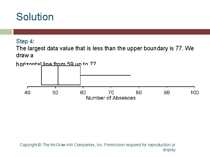
Solution Step 4: The largest data value that is less than the upper boundary is 77. We draw a horizontal line from 59 up to 77. Copyright © The Mc. Graw-Hill Companies, Inc. Permission required for reproduction or display.

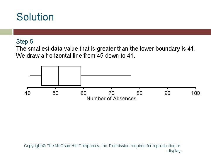
Solution Step 5: The smallest data value that is greater than the lower boundary is 41. We draw a horizontal line from 45 down to 41. Copyright © The Mc. Graw-Hill Companies, Inc. Permission required for reproduction or display.

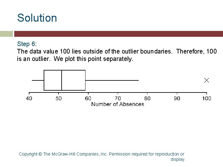
Solution Step 6: The data value 100 lies outside of the outlier boundaries. Therefore, 100 is an outlier. We plot this point separately. Copyright © The Mc. Graw-Hill Companies, Inc. Permission required for reproduction or display.

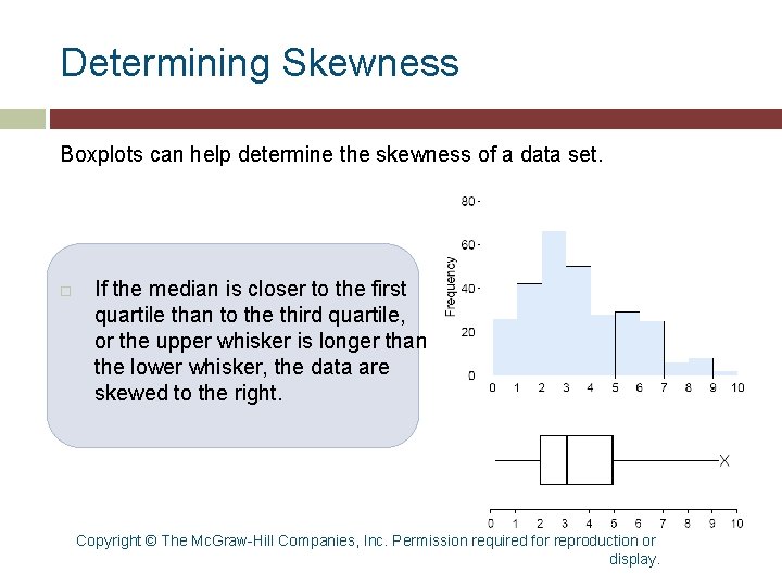
Determining Skewness Boxplots can help determine the skewness of a data set. If the median is closer to the first quartile than to the third quartile, or the upper whisker is longer than the lower whisker, the data are skewed to the right. Copyright © The Mc. Graw-Hill Companies, Inc. Permission required for reproduction or display.

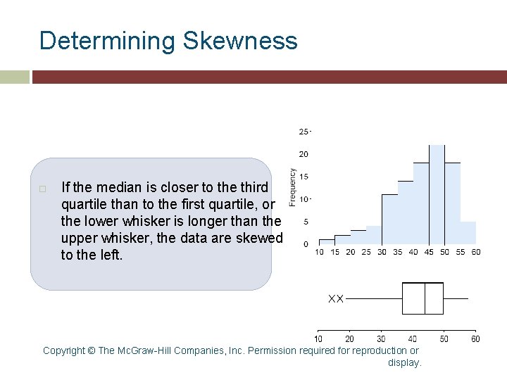
Determining Skewness If the median is closer to the third quartile than to the first quartile, or the lower whisker is longer than the upper whisker, the data are skewed to the left. Copyright © The Mc. Graw-Hill Companies, Inc. Permission required for reproduction or display.

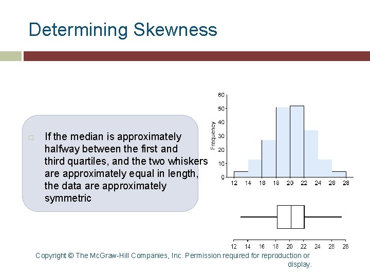
Determining Skewness If the median is approximately halfway between the first and third quartiles, and the two whiskers are approximately equal in length, the data are approximately symmetric Copyright © The Mc. Graw-Hill Companies, Inc. Permission required for reproduction or display.

Do You Know… • • • How to compute and interpret z-scores? How to compute percentiles of a data set? How to compute the quartiles of a data set? How to compute the five-number summary for a data set? The effects of outliers? How to construct boxplots? Copyright © The Mc. Graw-Hill Companies, Inc. Permission required for reproduction or display.