Copyright c2014 John Wiley Sons Inc Chapter 12

Copyright (c)2014 John Wiley & Sons, Inc. Chapter 12 Capturing Surplus 1

Chapter Twelve Overview 2. Price Discrimination • First Degree • Second Degree • Third Degree 3. Tie-in Sales • Requirements Tie-ins • Package Tie-ins (Bundling) Chapter Twelve Copyright (c)2014 John Wiley & Sons, Inc. 1. Introduction: Airline Tickets 2

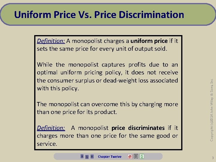
Uniform Price Vs. Price Discrimination While the monopolist captures profits due to an optimal uniform pricing policy, it does not receive the consumer surplus or dead-weight loss associated with this policy. The monopolist can overcome this by charging more than one price for its product. Definition: A monopolist price discriminates if it charges more than one price for the same good or service. Chapter Twelve Copyright (c)2014 John Wiley & Sons, Inc. Definition: A monopolist charges a uniform price if it sets the same price for every unit of output sold. 3

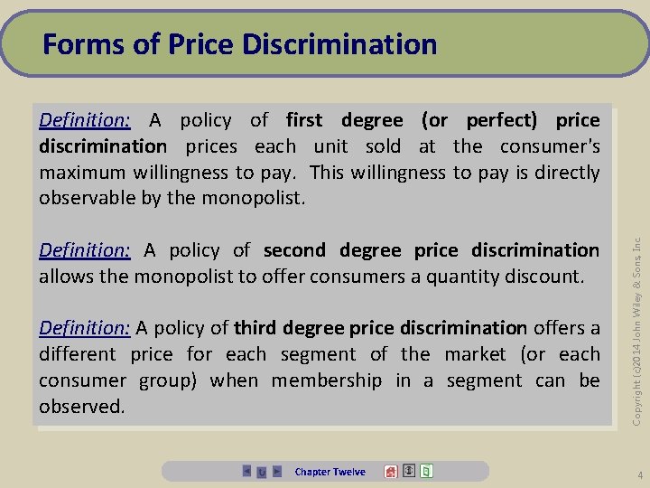
Forms of Price Discrimination Definition: A policy of second degree price discrimination allows the monopolist to offer consumers a quantity discount. Definition: A policy of third degree price discrimination offers a different price for each segment of the market (or each consumer group) when membership in a segment can be observed. Chapter Twelve Copyright (c)2014 John Wiley & Sons, Inc. Definition: A policy of first degree (or perfect) price discrimination prices each unit sold at the consumer's maximum willingness to pay. This willingness to pay is directly observable by the monopolist. 4

“Willingness to Pay” Curve Think of the demand curve as a "willingness to pay" curve. If the monopolist can observe the willingness to pay of each customer (based on, for example, residence, education, "look", etc), then the monopolist can observe demand perfectly and can "perfectly" price discriminate. Chapter Twelve Copyright (c)2014 John Wiley & Sons, Inc. Definition: The consumer's maximum willingness to pay is called the consumer's reservation price. 5

Definition: A policy of first degree (or perfect) price discrimination prices each unit sold at the consumer's maximum willingness to pay. This willingness to pay is directly observable by the monopolist. Chapter Twelve Copyright (c)2014 John Wiley & Sons, Inc. Forms of Price Discrimination 6

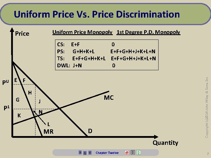
Uniform Price Vs. Price Discrimination Uniform Price Monopoly 1 st Degree P. D. Monopoly Price Copyright (c)2014 John Wiley & Sons, Inc. CS: E+F 0 PS: G+H+K+L E+F+G+H+J+K+L+N TS: E+F+G+H+K+L E+F+G+H+J+K+L+N DWL: J+N 0 PU E F G P 1 K H MC J N L MR D Quantity Chapter Twelve 7

Is it Reasonable? Therefore, a perfectly price discriminating monopolist will produce and sell the efficient quantity of output. Note: Only if the monopolist can prevent resale can the monopolist capture the entire surplus. Chapter Twelve Copyright (c)2014 John Wiley & Sons, Inc. The monopolist will continue selling units until the reservation price exactly equals marginal cost. 8

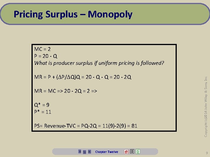
Pricing Surplus – Monopoly MR = P + ( P/ Q)Q = 20 - 2 Q MR = MC => 20 - 2 Q = 2 => Q* = 9 P* = 11 PS= Revenue-TVC = PQ-2 Q = 11(9)-2(9) = 81 Chapter Twelve Copyright (c)2014 John Wiley & Sons, Inc. MC = 2 P = 20 - Q What is producer surplus if uniform pricing is followed? 9

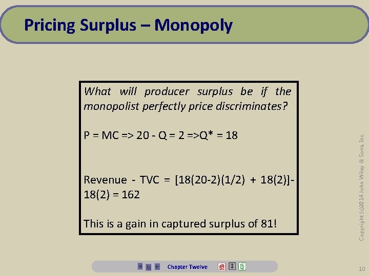
Pricing Surplus – Monopoly P = MC => 20 - Q = 2 =>Q* = 18 Revenue - TVC = [18(20 -2)(1/2) + 18(2)]18(2) = 162 This is a gain in captured surplus of 81! Chapter Twelve Copyright (c)2014 John Wiley & Sons, Inc. What will producer surplus be if the monopolist perfectly price discriminates? 10

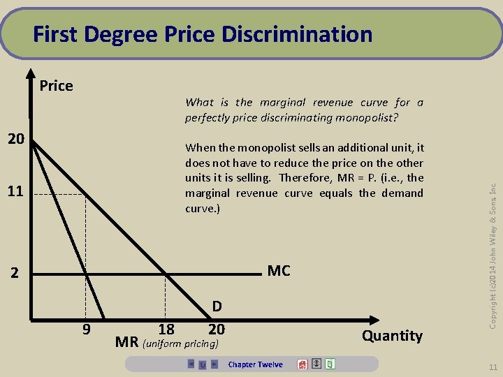
First Degree Price Discrimination Price 20 When the monopolist sells an additional unit, it does not have to reduce the price on the other units it is selling. Therefore, MR = P. (i. e. , the marginal revenue curve equals the demand curve. ) 11 MC 2 9 18 D 20 Quantity MR (uniform pricing) Chapter Twelve Copyright (c)2014 John Wiley & Sons, Inc. What is the marginal revenue curve for a perfectly price discriminating monopolist? 11

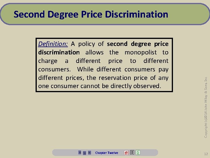
Definition: A policy of second degree price discrimination allows the monopolist to charge a different price to different consumers. While different consumers pay different prices, the reservation price of any one consumer cannot be directly observed. Chapter Twelve Copyright (c)2014 John Wiley & Sons, Inc. Second Degree Price Discrimination 12

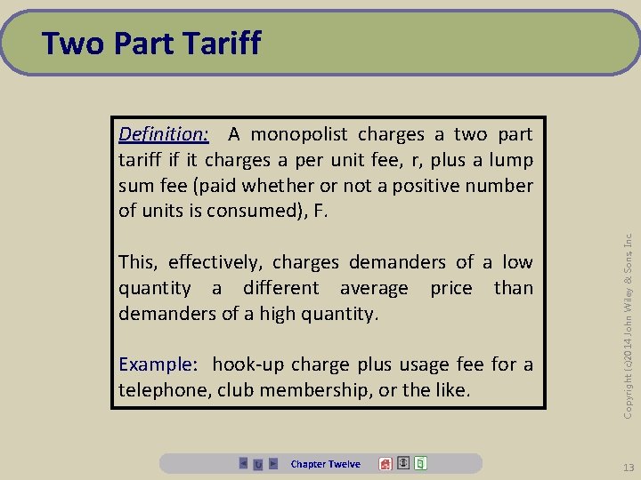
Two Part Tariff This, effectively, charges demanders of a low quantity a different average price than demanders of a high quantity. Example: hook-up charge plus usage fee for a telephone, club membership, or the like. Chapter Twelve Copyright (c)2014 John Wiley & Sons, Inc. Definition: A monopolist charges a two part tariff if it charges a per unit fee, r, plus a lump sum fee (paid whether or not a positive number of units is consumed), F. 13

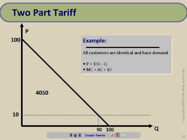
Two Part Tariff P 100 Example: All customers are identical and have demand Copyright (c)2014 John Wiley & Sons, Inc. • P = 100 - Q • MC = AC = 10 4050 10 90 100 Chapter Twelve Q 14

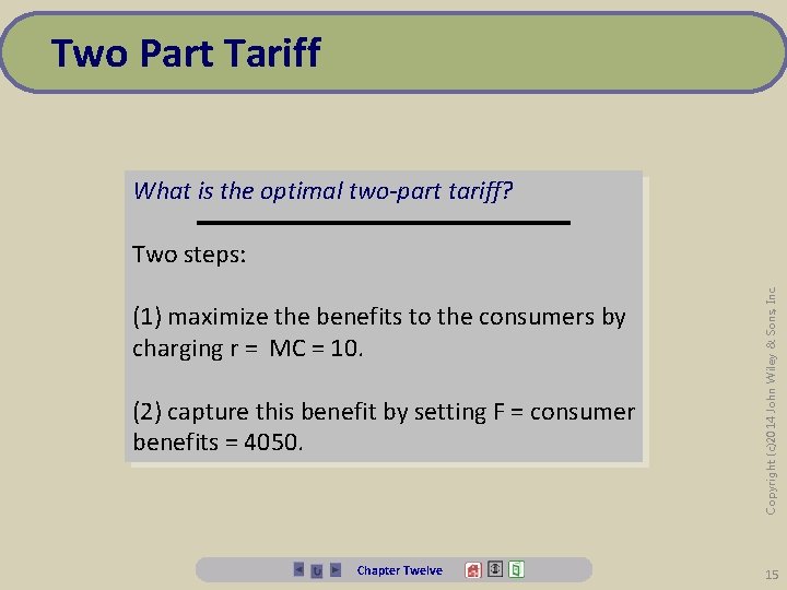
Two Part Tariff What is the optimal two-part tariff? (1) maximize the benefits to the consumers by charging r = MC = 10. (2) capture this benefit by setting F = consumer benefits = 4050. Chapter Twelve Copyright (c)2014 John Wiley & Sons, Inc. Two steps: 15

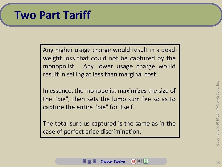
Two Part Tariff In essence, the monopolist maximizes the size of the "pie", then sets the lump sum fee so as to capture the entire "pie" for itself. The total surplus captured is the same as in the case of perfect price discrimination. Chapter Twelve Copyright (c)2014 John Wiley & Sons, Inc. Any higher usage charge would result in a deadweight loss that could not be captured by the monopolist. Any lower usage charge would result in selling at less than marginal cost. 16

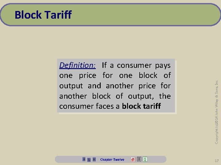
Definition: If a consumer pays one price for one block of output and another price for another block of output, the consumer faces a block tariff Chapter Twelve Copyright (c)2014 John Wiley & Sons, Inc. Block Tariff 17

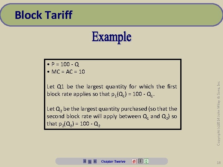
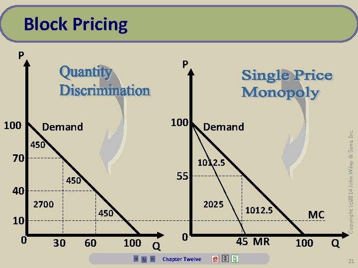
Block Tariff Let Q 1 be the largest quantity for which the first block rate applies so that p 1(Q 1) = 100 - Q 1. Let Q 2 be the largest quantity purchased (so that the second block rate will apply between Q 1 and Q 2) so that p 2(Q 2) = 100 - Q 2 Chapter Twelve Copyright (c)2014 John Wiley & Sons, Inc. • P = 100 - Q • MC = AC = 10 18

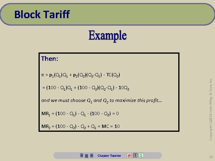
Block Tariff = p 1(Q 1)Q 1 + p 2(Q 2)(Q 2 -Q 1) - TC(Q 2) = (100 - Q 1)Q 1 + (100 - Q 2)(Q 2 -Q 1) - 10 Q 2 and we must choose Q 1 and Q 2 to maximize this profit… MR 1 = (100 - Q 1) - Q 1 - (100 - Q 2) = 0 MR 2 = (100 - Q 2) - Q 2 + Q 1 = MC = 10 Chapter Twelve Copyright (c)2014 John Wiley & Sons, Inc. Then: 19

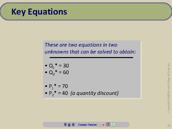
Key Equations • Q 1* = 30 • Q 2* = 60 • P 1* = 70 • P 2* = 40 (a quantity discount) Chapter Twelve Copyright (c)2014 John Wiley & Sons, Inc. These are two equations in two unknowns that can be solved to obtain: 20

Block Pricing P 70 100 Demand 450 55 450 40 2700 30 1012. 5 2025 450 10 0 Demand Copyright (c)2014 John Wiley & Sons, Inc. 100 P 60 100 Q 0 Chapter Twelve 1012. 5 45 MR MC 100 Q 21

If the monopolist could set a different block price for each customer, it would capture the same amount of surplus as a perfectly price discriminating monopolist. Chapter Twelve Copyright (c)2014 John Wiley & Sons, Inc. Block Pricing 22

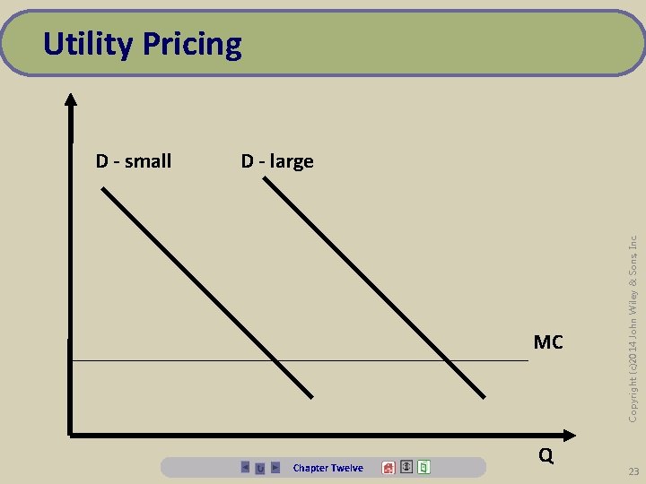
Utility Pricing D - large MC Chapter Twelve Q Copyright (c)2014 John Wiley & Sons, Inc. D - small 23

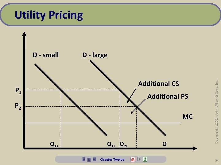
Utility Pricing D - large Additional CS P 1 Additional PS P 2 MC Q 1 s Q 1 L Q 2 L Chapter Twelve Q Copyright (c)2014 John Wiley & Sons, Inc. D - small 24

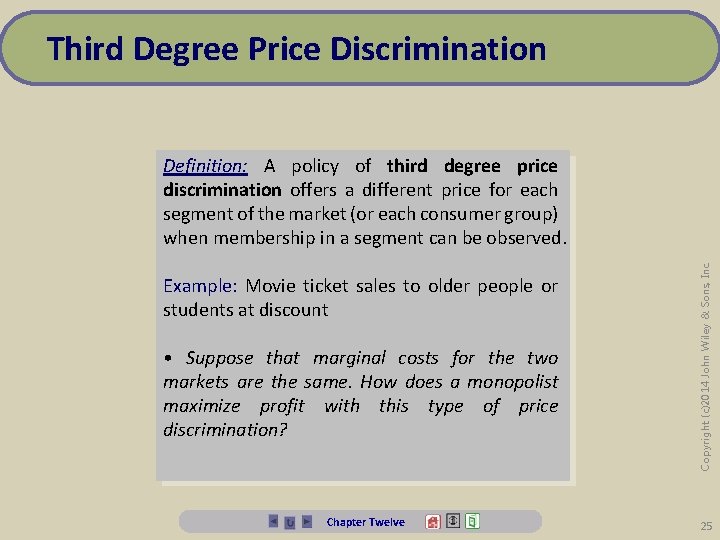
Third Degree Price Discrimination Example: Movie ticket sales to older people or students at discount • Suppose that marginal costs for the two markets are the same. How does a monopolist maximize profit with this type of price discrimination? Chapter Twelve Copyright (c)2014 John Wiley & Sons, Inc. Definition: A policy of third degree price discrimination offers a different price for each segment of the market (or each consumer group) when membership in a segment can be observed. 25

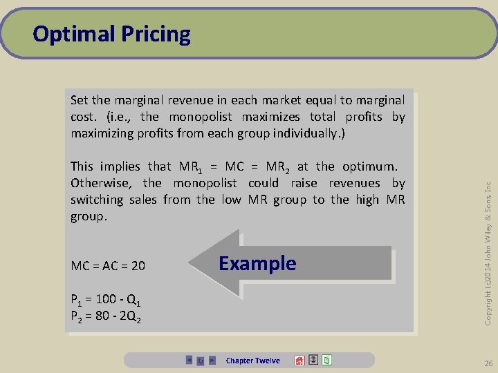
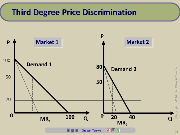
Optimal Pricing This implies that MR 1 = MC = MR 2 at the optimum. Otherwise, the monopolist could raise revenues by switching sales from the low MR group to the high MR group. MC = AC = 20 Example P 1 = 100 - Q 1 P 2 = 80 - 2 Q 2 Chapter Twelve Copyright (c)2014 John Wiley & Sons, Inc. Set the marginal revenue in each market equal to marginal cost. (i. e. , the monopolist maximizes total profits by maximizing profits from each group individually. ) 26

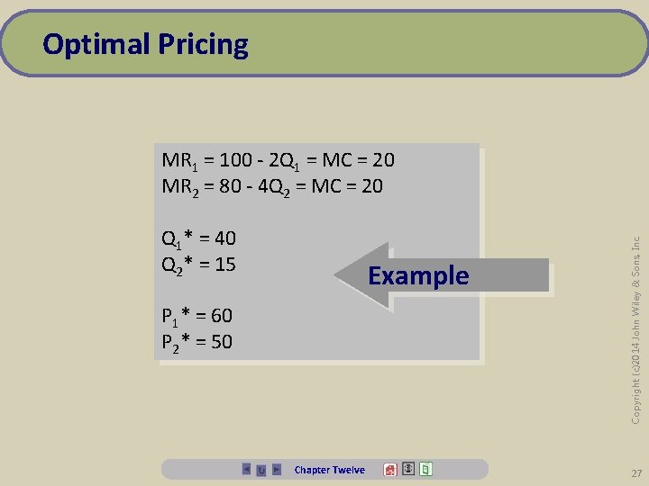
Optimal Pricing Q 1* = 40 Q 2* = 15 Example P 1* = 60 P 2* = 50 Chapter Twelve Copyright (c)2014 John Wiley & Sons, Inc. MR 1 = 100 - 2 Q 1 = MC = 20 MR 2 = 80 - 4 Q 2 = MC = 20 27

Third Degree Price Discrimination Market 1 P 100 Demand 1 80 60 Market 2 Demand 2 50 20 0 MR 1 100 Q 0 Chapter Twelve 20 40 MR 2 Q Copyright (c)2014 John Wiley & Sons, Inc. P 28

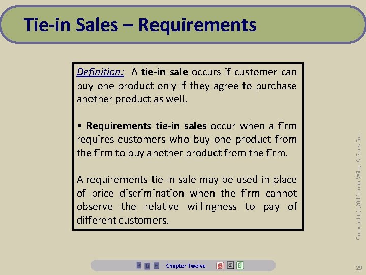
Tie-in Sales – Requirements • Requirements tie-in sales occur when a firm requires customers who buy one product from the firm to buy another product from the firm. A requirements tie-in sale may be used in place of price discrimination when the firm cannot observe the relative willingness to pay of different customers. Chapter Twelve Copyright (c)2014 John Wiley & Sons, Inc. Definition: A tie-in sale occurs if customer can buy one product only if they agree to purchase another product as well. 29

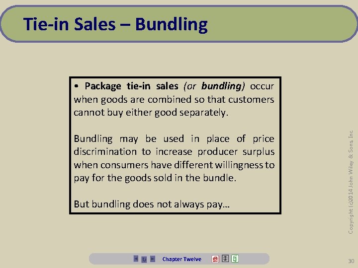
Tie-in Sales – Bundling may be used in place of price discrimination to increase producer surplus when consumers have different willingness to pay for the goods sold in the bundle. But bundling does not always pay… Chapter Twelve Copyright (c)2014 John Wiley & Sons, Inc. • Package tie-in sales (or bundling) occur when goods are combined so that customers cannot buy either good separately. 30

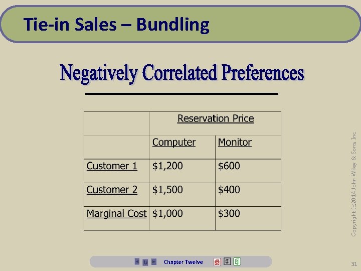
Copyright (c)2014 John Wiley & Sons, Inc. Tie-in Sales – Bundling Chapter Twelve 31

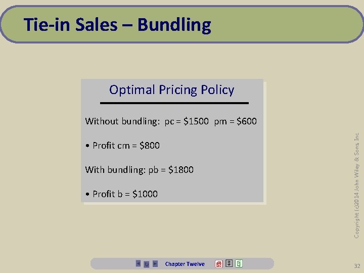
Tie-in Sales – Bundling Optimal Pricing Policy • Profit cm = $800 With bundling: pb = $1800 • Profit b = $1000 Chapter Twelve Copyright (c)2014 John Wiley & Sons, Inc. Without bundling: pc = $1500 pm = $600 32

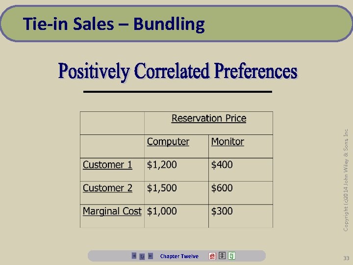
Copyright (c)2014 John Wiley & Sons, Inc. Tie-in Sales – Bundling Chapter Twelve 33

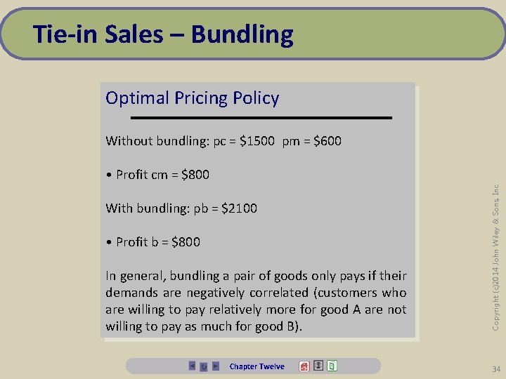
Tie-in Sales – Bundling Optimal Pricing Policy Without bundling: pc = $1500 pm = $600 With bundling: pb = $2100 • Profit b = $800 In general, bundling a pair of goods only pays if their demands are negatively correlated (customers who are willing to pay relatively more for good A are not willing to pay as much for good B). Chapter Twelve Copyright (c)2014 John Wiley & Sons, Inc. • Profit cm = $800 34

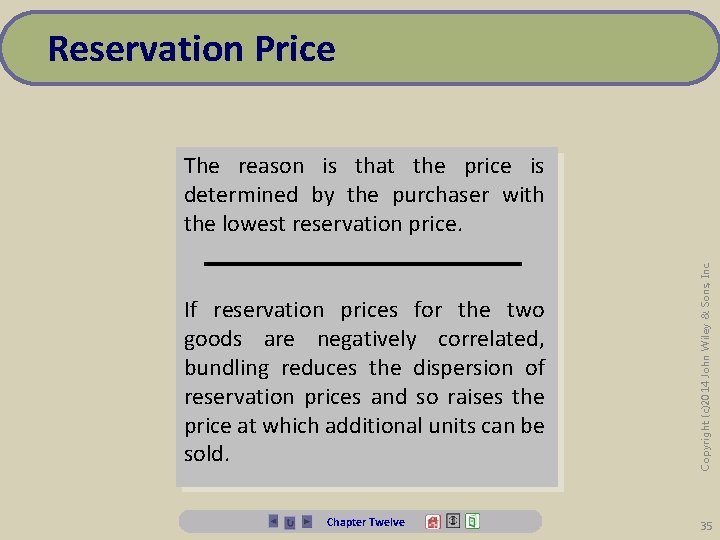
Reservation Price If reservation prices for the two goods are negatively correlated, bundling reduces the dispersion of reservation prices and so raises the price at which additional units can be sold. Copyright (c)2014 John Wiley & Sons, Inc. The reason is that the price is determined by the purchaser with the lowest reservation price. Chapter Twelve 35

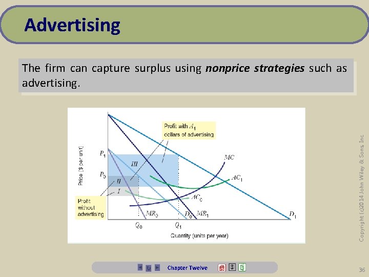
Advertising Copyright (c)2014 John Wiley & Sons, Inc. The firm can capture surplus using nonprice strategies such as advertising. Chapter Twelve 36