COP 4710 Database Systems Fall 2012 Chapter 4

COP 4710: Database Systems Fall 2012 Chapter 4 – Relational Query Languages – Part 2 Instructor : Dr. Mark Llewellyn markl@cs. ucf. edu HEC 236, 407 -823 -2790 http: //www. cs. ucf. edu/courses/cop 4710/fall 2012 Department of Electrical Engineering and Computer Science Division University of Central Florida COP 4710: Database Systems (Chapter 4) Page 1 Dr.

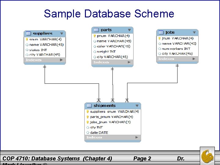
Sample Database Scheme COP 4710: Database Systems (Chapter 4) Page 2 Dr.

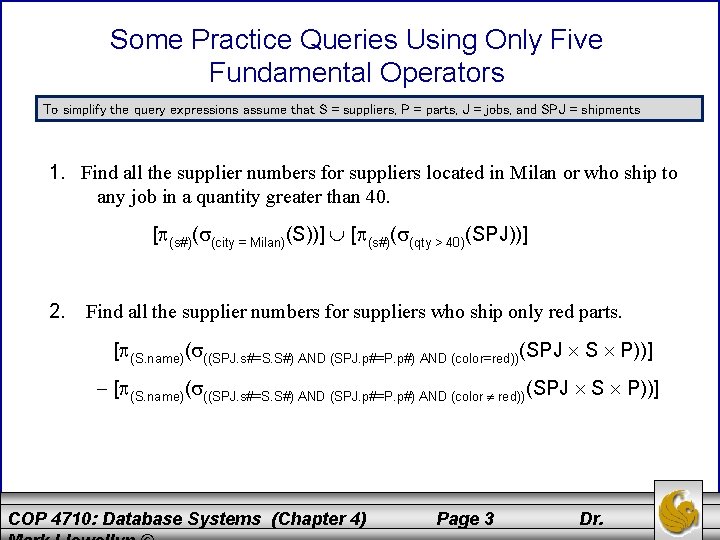
Some Practice Queries Using Only Five Fundamental Operators To simplify the query expressions assume that S = suppliers, P = parts, J = jobs, and SPJ = shipments 1. Find all the supplier numbers for suppliers located in Milan or who ship to any job in a quantity greater than 40. [ (s#)( (city = Milan)(S))] [ (s#)( (qty > 40)(SPJ))] 2. Find all the supplier numbers for suppliers who ship only red parts. [ (S. name)( ((SPJ. s#=S. S#) AND (SPJ. p#=P. p#) AND (color=red))(SPJ S P))] [ (S. name)( ((SPJ. s#=S. S#) AND (SPJ. p#=P. p#) AND (color red))(SPJ S P))] COP 4710: Database Systems (Chapter 4) Page 3 Dr.

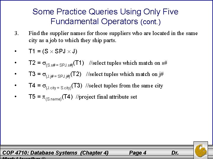
Some Practice Queries Using Only Five Fundamental Operators (cont. ) 3. Find the supplier names for those suppliers who are located in the same city as a job to which they ship parts. • T 1 = (S SPJ J) • T 2 = (S. s# = SPJ. s#)(T 1) //select tuples which match on s# • T 3 = (J. j# = SPJ. j#)(T 2) //select tuples which match on j# • T 4 = (J. city = S. city)(T 3) //select tuples from the same city • T 5 = (S. name)(T 4) //project final attribute set COP 4710: Database Systems (Chapter 4) Page 4 Dr.

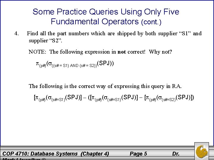
Some Practice Queries Using Only Five Fundamental Operators (cont. ) 4. Find all the part numbers which are shipped by both supplier “S 1” and supplier “S 2”. NOTE: The following expression in not correct! Why not? (p#)( ((s# = S 1) AND (s# = S 2))(SPJ)) The following is the correct way of expressing this query in RA. [ (p#)( (s#=S 1)(SPJ)] – ([ (p#)( (s#=S 1)(SPJ)] [ (p#)( (s#=S 2)(SPJ)]) COP 4710: Database Systems (Chapter 4) Page 5 Dr.

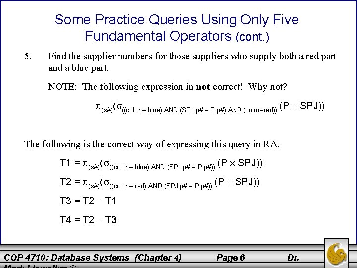
Some Practice Queries Using Only Five Fundamental Operators (cont. ) 5. Find the supplier numbers for those suppliers who supply both a red part and a blue part. NOTE: The following expression in not correct! Why not? (s#)( ((color = blue) AND (SPJ. p# = P. p#) AND (color=red)) (P SPJ)) The following is the correct way of expressing this query in RA. T 1 = (s#)( ((color = blue) AND (SPJ. p# = P. p#)) (P SPJ)) T 2 = (s#)( ((color = red) AND (SPJ. p# = P. p#)) (P SPJ)) T 3 = T 2 – T 1 T 4 = T 2 – T 3 COP 4710: Database Systems (Chapter 4) Page 6 Dr.

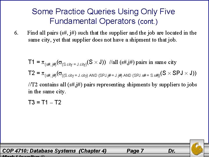
Some Practice Queries Using Only Five Fundamental Operators (cont. ) 6. Find all pairs (s#, j#) such that the supplier and the job are located in the same city, yet that supplier does not have a shipment to that job. T 1 = (s#, j#)( (S. city = J. city)(S J)) //all (s#, j#) pairs in same city T 2 = (s#, j#)( ((S. city = J. city) AND (SPJ. j# = J. j#) AND (SPJ. s# = S. s#))(S SPJ J)) //T 2 contains all (s#, j#) pairs representing shipments by suppliers to jobs in the same city. T 3 = T 1 – T 2 COP 4710: Database Systems (Chapter 4) Page 7 Dr.

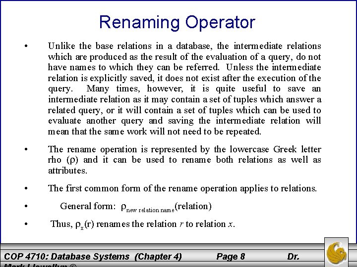
Renaming Operator • Unlike the base relations in a database, the intermediate relations which are produced as the result of the evaluation of a query, do not have names to which they can be referred. Unless the intermediate relation is explicitly saved, it does not exist after the execution of the query. Many times, however, it is quite useful to save an intermediate relation as it may contain a set of tuples which answer a related query, or it will contain a set of tuples which can be used to evaluate another query and saving the intermediate relation will mean that the same work will not need to be repeated. • The rename operation is represented by the lowercase Greek letter rho ( ) and it can be used to rename both relations as well as attributes. • The first common form of the rename operation applies to relations. • • General form: new relation name(relation) Thus, x(r) renames the relation r to relation x. COP 4710: Database Systems (Chapter 4) Page 8 Dr.

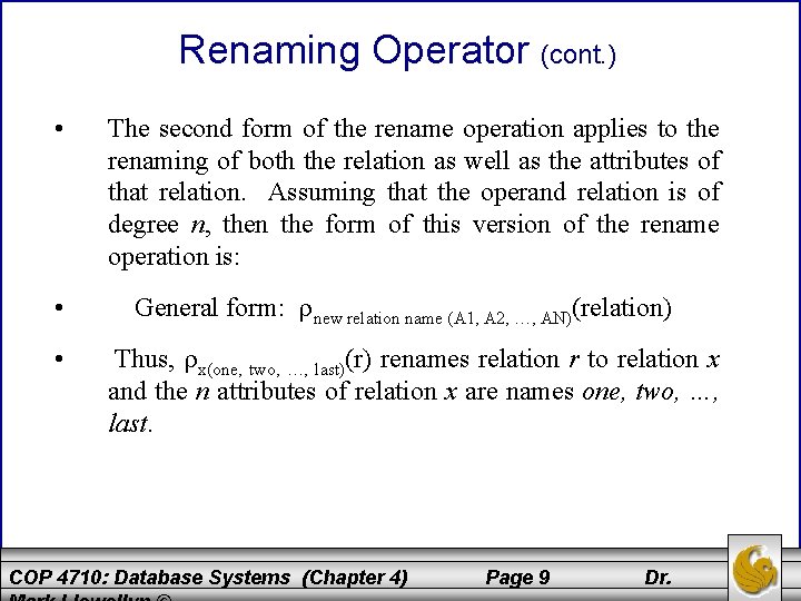
Renaming Operator (cont. ) • • • The second form of the rename operation applies to the renaming of both the relation as well as the attributes of that relation. Assuming that the operand relation is of degree n, then the form of this version of the rename operation is: General form: new relation name (A 1, A 2, …, AN)(relation) Thus, x(one, two, …, last)(r) renames relation r to relation x and the n attributes of relation x are names one, two, …, last. COP 4710: Database Systems (Chapter 4) Page 9 Dr.

Redundant Operators in Relational Algebra • It can be proven (although we aren’t going to go through that proof) that the five fundamental relational operations are sufficient to express any relational-algebra query. • What this proof doesn’t state however, is that some complex queries will require extremely lengthy and difficult query expressions. • There have been several extensions of the set of operations available in the relational algebra that provide no additional expressive power, but do provide a simplification in the expression required for more complex queries. • We’ll look at the most important and common of these redundant operations and also show their definition in terms of the five fundamental operations COP 4710: Database Systems (Chapter 4) Page 10 Dr.

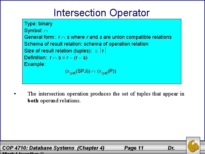
Intersection Operator Type: binary Symbol: General form: r s where r and s are union compatible relations Schema of result relation: schema of operation relation Size of result relation (tuples): r Definition: r s r (r s) Example: ( (p#)(SPJ)) ( (p#)(P)) • The intersection operation produces the set of tuples that appear in both operand relations. COP 4710: Database Systems (Chapter 4) Page 11 Dr.

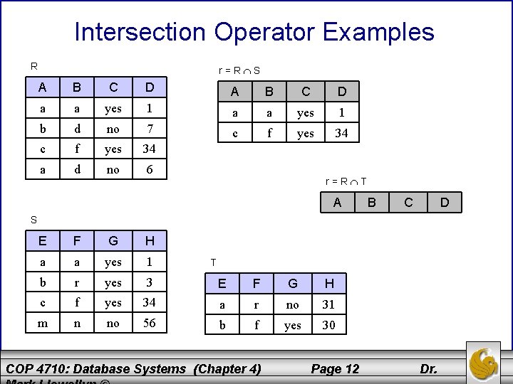
Intersection Operator Examples R r=R S A B C D a a yes 1 b d no 7 c f yes 34 a d no 6 r=R T A B C D S E F G H a a yes 1 b r yes 3 E F G H c f yes 34 a r no 31 m n no 56 b f yes 30 T COP 4710: Database Systems (Chapter 4) Page 12 Dr.

Join Operators • As we saw in some of our earlier query expression which involved the Cartesian product operator, we had to provide additional selection operations to remove those combinations of tuples that resulted from the Cartesian product which weren’t related (they didn’t make sense like when a shipment of a specific part was combined with part information but the part information didn’t belong to the part that was being shipped). • This occurs so commonly that an operation which is a combination of the Cartesian product and selection operations was developed called a join operation. • There are several different join operations which are called, thetajoin, equijoin, natural join, outer join, and semijoin. We will examine each of these operations and explore the conditions of their use. COP 4710: Database Systems (Chapter 4) Page 13 Dr.

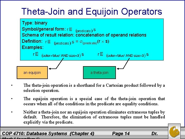
Theta-Join and Equijoin Operators Type: binary Symbol/general form: Schema of result relation: concatenation of operand relations Definition: (predicate)(r s) Examples: an equijoin a theta-join • The theta-join operation is a shorthand for a Cartesian product followed by a selection operation. • The equijoin operation is a special case of theta-join operation that occurs when all of the conditions in the predicate are equality conditions. • Neither a theta-join nor an equijoin operation eliminates extraneous tuples by default. Therefore, the elimination of extraneous tuples must be handled explicitly via the predicate. COP 4710: Database Systems (Chapter 4) Page 14 Dr.

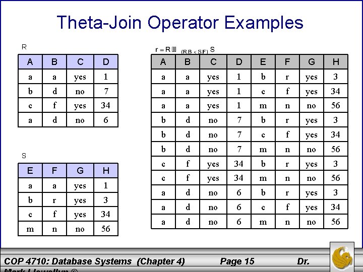
Theta-Join Operator Examples R A B C D E F G H a a yes 1 b r yes 3 b d no 7 a a yes 1 c f yes 34 a a yes 1 m n no 56 a d no 6 b d no 7 b r yes 3 b d no 7 c f yes 34 b d no 7 m n no 56 c f yes 34 b r yes 3 c f yes 34 m n no 56 a d no 6 b r yes 3 a d no 6 c f yes 34 a d no 6 m n no 56 S E F G H a a yes 1 b r yes 3 c f yes 34 m n no 56 COP 4710: Database Systems (Chapter 4) Page 15 Dr.

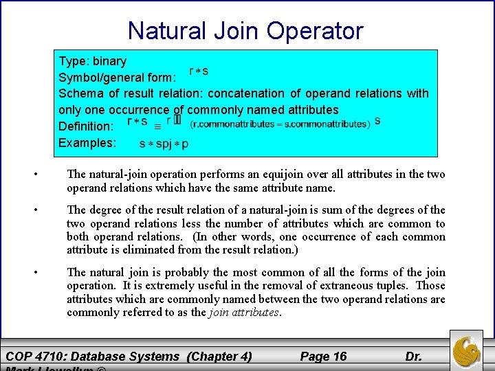
Natural Join Operator Type: binary Symbol/general form: Schema of result relation: concatenation of operand relations with only one occurrence of commonly named attributes Definition: Examples: • The natural-join operation performs an equijoin over all attributes in the two operand relations which have the same attribute name. • The degree of the result relation of a natural-join is sum of the degrees of the two operand relations less the number of attributes which are common to both operand relations. (In other words, one occurrence of each common attribute is eliminated from the result relation. ) • The natural join is probably the most common of all the forms of the join operation. It is extremely useful in the removal of extraneous tuples. Those attributes which are commonly named between the two operand relations are commonly referred to as the join attributes. COP 4710: Database Systems (Chapter 4) Page 16 Dr.

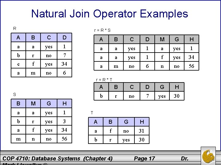
Natural Join Operator Examples R r=R*S A B C D M G H a a yes 1 b r no 7 a a yes 1 f yes 34 c f yes 34 a m no 6 n no 56 a m no 6 A B C D G H b r no 7 yes 30 r=R*T S B M G H a a yes 1 b r yes 3 A B G H a f yes 34 a f no 31 m n no 56 b r yes 30 T COP 4710: Database Systems (Chapter 4) Page 17 Dr.

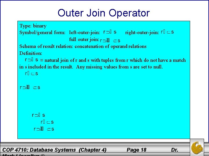
Outer Join Operator Type: binary Symbol/general form: left-outer-join: right-outer-join: full outer join: Schema of result relation: concatenation of operand relations Definition: natural join of r and s with tuples from r which do not have a match in s included in the result. Any missing values from s are set to null. COP 4710: Database Systems (Chapter 4) Page 18 Dr.

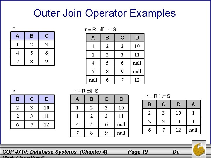
Outer Join Operator Examples R A B C D 1 2 3 10 4 5 6 1 2 3 11 7 8 9 4 5 6 null 7 8 9 null 6 7 12 S B C D A B C D 2 3 10 1 2 3 10 2 3 11 1 2 3 11 6 7 12 4 5 6 null 7 8 9 null COP 4710: Database Systems (Chapter 4) B C D A 2 3 10 1 2 3 11 1 6 7 12 null Page 19 Dr.

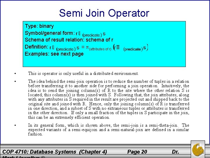
Semi Join Operator c Type: binary Symbol/general form: Schema of result relation: schema of r Definition: (attributes of r) Examples: see next page • This is operator is only useful in a distributed environment. • The idea behind the semi-join operation is to reduce the number of tuples in a relation before transferring it to another side for performing a join operation. Intuitively, the idea is to send the joining column(s) of R to the site where the other relation S is located; this column(s) is then joined with S. Following that, the join attributes, along with any attributes in S required in the result are projected out and shipped back to the original site and joined with R. Hence, only the joining column(s) of R is transferred in one direction, and a subset of S with no extraneous tuples or attributes is transferred in the other direction. If only a small fraction of the tuples in S participate in the join, this can be an extremely efficient operation. • In its general form, which is shown above, the semi-join is a semi-theta-join. The expected variants of a semi-equijoin and a semi-natural-join are defined in a similar fashion. COP 4710: Database Systems (Chapter 4) Page 20 Dr.

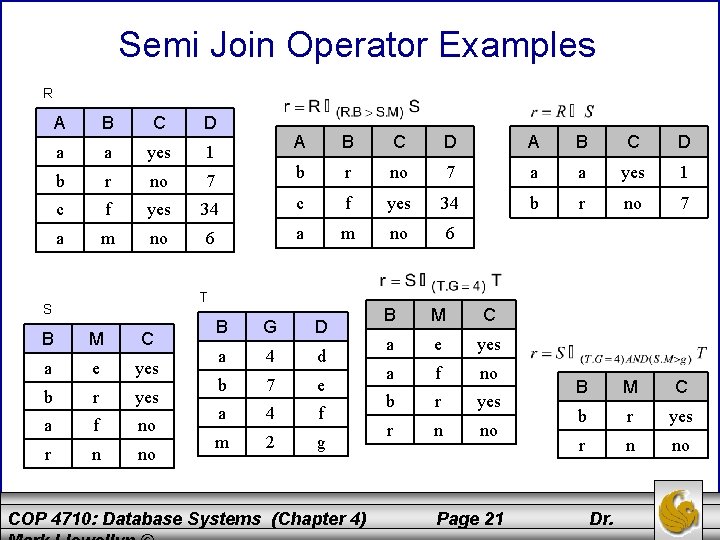
Semi Join Operator Examples R A B C D a a yes 1 b r no c f a m A B C D 7 b r no 7 a a yes 1 yes 34 c f yes 34 b r no 7 no 6 a m no 6 B M C b r yes r n no T S B M C a e yes b r yes a f no r n no B G D a 4 d b 7 e a 4 f m 2 g COP 4710: Database Systems (Chapter 4) B M C a e yes a f no b r yes r n no Page 21 Dr.

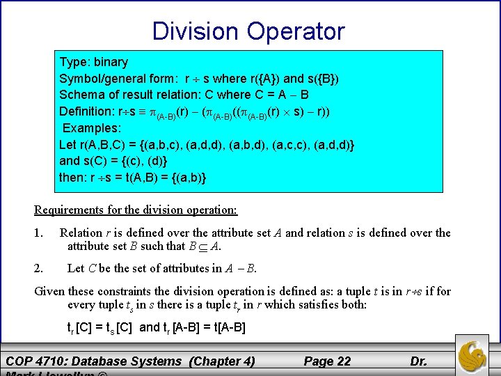
Division Operator c Type: binary Symbol/general form: r s where r({A}) and s({B}) Schema of result relation: C where C = A B Definition: r s (A-B)(r) ( (A-B)(r) s) r)) Examples: Let r(A, B, C) = {(a, b, c), (a, d, d), (a, b, d), (a, c, c), (a, d, d)} and s(C) = {(c), (d)} then: r s = t(A, B) = {(a, b)} Requirements for the division operation: 1. 2. Relation r is defined over the attribute set A and relation s is defined over the attribute set B such that B A. Let C be the set of attributes in A B. Given these constraints the division operation is defined as: a tuple t is in r s if for every tuple ts in s there is a tuple tr in r which satisfies both: tr [C] = ts [C] and tr [A-B] = t[A-B] COP 4710: Database Systems (Chapter 4) Page 22 Dr.

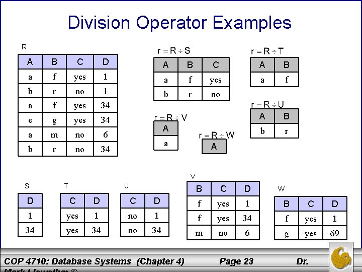
Division Operator Examples R A B C D A B C A B a f yes 1 a f yes a f b r no 1 b r no a f yes 34 e g yes 34 A B a m no 6 b r no 34 A a A V S T U B C D W D C D f yes 1 B C D 1 yes 1 no 1 f yes 34 f yes 1 34 yes 34 no 34 m no 6 g yes 69 COP 4710: Database Systems (Chapter 4) Page 23 Dr.

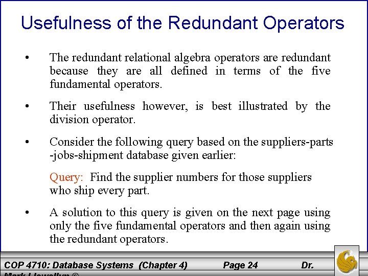
Usefulness of the Redundant Operators • The redundant relational algebra operators are redundant because they are all defined in terms of the five fundamental operators. • Their usefulness however, is best illustrated by the division operator. • Consider the following query based on the suppliers-parts -jobs-shipment database given earlier: Query: Find the supplier numbers for those suppliers who ship every part. • A solution to this query is given on the next page using only the five fundamental operators and then again using the redundant operators. COP 4710: Database Systems (Chapter 4) Page 24 Dr.

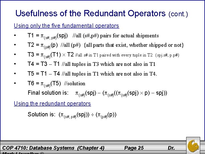
Usefulness of the Redundant Operators (cont. ) Using only the five fundamental operators • T 1 = (s#, p#)(spj) //all (s#, p#) pairs for actual shipments • T 2 = (p#)(p) //all (p#) {all parts that exist, whether shipped or not} • T 3 = (s#)(T 1) T 2 //all s# in T 1 paired with every tuple in T 2 • T 4 = T 3 – T 1 //all tuples in T 3 which are not also in T 1 • T 5 = T 1 – T 4 //all tuples in T 1 which are not also in T 4. • T 6 = (s#)(T 5) //solution Final solution is: {spj. s#, p. p#} (s#)(spj) ( (s#)(spj) p) spj)) Using the redundant operators Solution is: ( (s#, p#)(spj)) ( (p#)(p)) COP 4710: Database Systems (Chapter 4) Page 25 Dr.

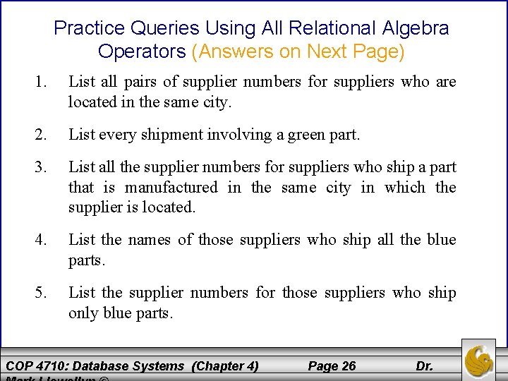
Practice Queries Using All Relational Algebra Operators (Answers on Next Page) 1. List all pairs of supplier numbers for suppliers who are located in the same city. 2. List every shipment involving a green part. 3. List all the supplier numbers for suppliers who ship a part that is manufactured in the same city in which the supplier is located. 4. List the names of those suppliers who ship all the blue parts. 5. List the supplier numbers for those suppliers who ship only blue parts. COP 4710: Database Systems (Chapter 4) Page 26 Dr.

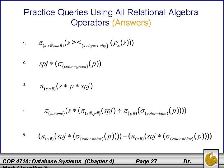
Practice Queries Using All Relational Algebra Operators (Answers) 1. 2. 3. 4. 5. COP 4710: Database Systems (Chapter 4) Page 27 Dr.

Tuple Relational Calculus • Relational algebra was a procedural query language. You specified in the query expression what data you wanted (this was usually given by the final projection) and you specified how the DBMS was to go about getting this data. The how was specified in the sequence of operations that you put together in order to answer your query. • Relational calculus is a non-procedural query language that has two basic forms: tuple relational calculus and domain relational calculus. While they are similar in nature there are fundamental differences in the two forms. • For now, we will focus on the tuple relational calculus. We won’t look at either of the calculus languages in quite the same detail that we did with the relational algebra, we’re more interested here in giving you an idea of what these pure languages look like since they form the foundation of the implemented languages such as SQL that we’ll see later. COP 4710: Database Systems (Chapter 4) Page 28 Dr.

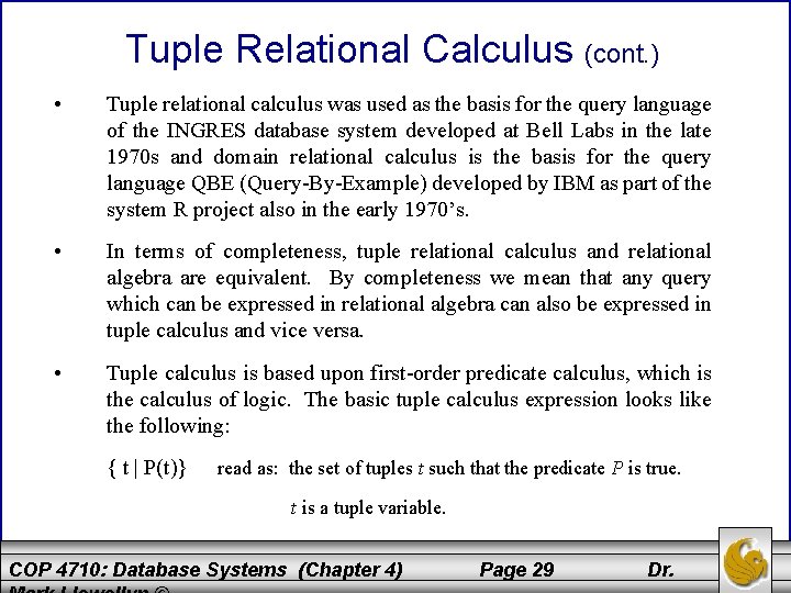
Tuple Relational Calculus (cont. ) • Tuple relational calculus was used as the basis for the query language of the INGRES database system developed at Bell Labs in the late 1970 s and domain relational calculus is the basis for the query language QBE (Query-By-Example) developed by IBM as part of the system R project also in the early 1970’s. • In terms of completeness, tuple relational calculus and relational algebra are equivalent. By completeness we mean that any query which can be expressed in relational algebra can also be expressed in tuple calculus and vice versa. • Tuple calculus is based upon first-order predicate calculus, which is the calculus of logic. The basic tuple calculus expression looks like the following: { t | P(t)} read as: the set of tuples t such that the predicate P is true. t is a tuple variable. COP 4710: Database Systems (Chapter 4) Page 29 Dr.

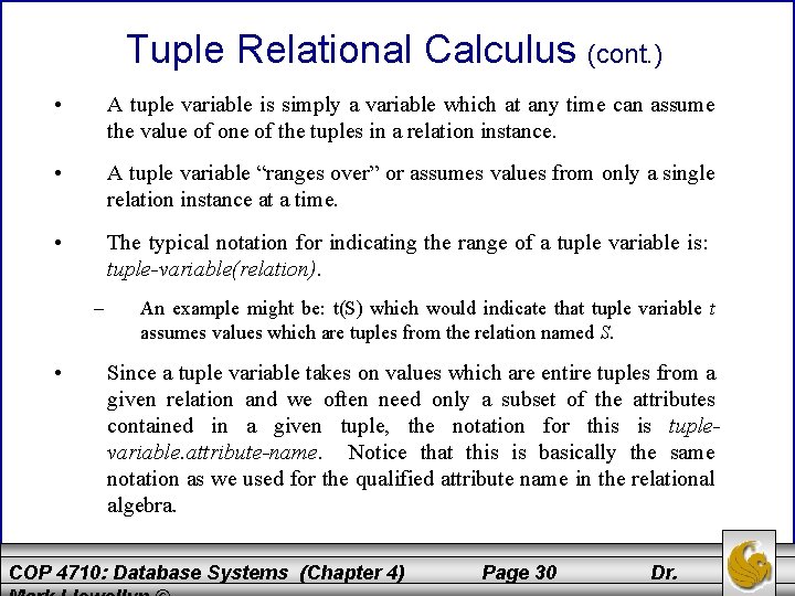
Tuple Relational Calculus (cont. ) • A tuple variable is simply a variable which at any time can assume the value of one of the tuples in a relation instance. • A tuple variable “ranges over” or assumes values from only a single relation instance at a time. • The typical notation for indicating the range of a tuple variable is: tuple-variable(relation). – • An example might be: t(S) which would indicate that tuple variable t assumes values which are tuples from the relation named S. Since a tuple variable takes on values which are entire tuples from a given relation and we often need only a subset of the attributes contained in a given tuple, the notation for this is tuplevariable. attribute-name. Notice that this is basically the same notation as we used for the qualified attribute name in the relational algebra. COP 4710: Database Systems (Chapter 4) Page 30 Dr.

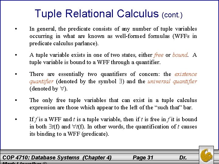
Tuple Relational Calculus (cont. ) • In general, the predicate consists of any number of tuple variables occurring in what are known as well-formed formulas (WFFs in predicate calculus parlance). • A tuple variable exists in one of two states, either free or bound. A tuple variable is bound to a WFF through a quantifier. • There are essentially two quantifiers of concern: the existence quantifier (denoted by the symbol ) and the universal quantifier (denoted by ). • The only free tuple variables that can exist in a tuple calculus expression are those which appear to the left of the “such that” bar. • If f is a WFF and t is a tuple variable, then if t is free in f it is bound in both t(f) and t(f). In other words, the quantification of t causes its binding to a WFF (predicate). COP 4710: Database Systems (Chapter 4) Page 31 Dr.

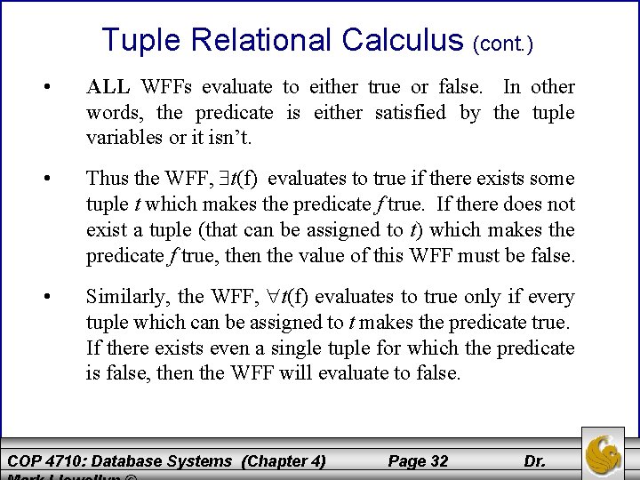
Tuple Relational Calculus (cont. ) • ALL WFFs evaluate to either true or false. In other words, the predicate is either satisfied by the tuple variables or it isn’t. • Thus the WFF, t(f) evaluates to true if there exists some tuple t which makes the predicate f true. If there does not exist a tuple (that can be assigned to t) which makes the predicate f true, then the value of this WFF must be false. • Similarly, the WFF, t(f) evaluates to true only if every tuple which can be assigned to t makes the predicate true. If there exists even a single tuple for which the predicate is false, then the WFF will evaluate to false. COP 4710: Database Systems (Chapter 4) Page 32 Dr.

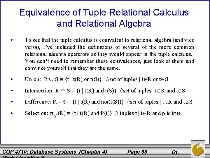
Equivalence of Tuple Relational Calculus and Relational Algebra • To see that the tuple calculus is equivalent to relational algebra (and vice versa), I’ve included the definitions of several of the more common relational algebra operators as they would appear in the tuple calculus. You don’t need to remember these equivalences, just look at them and convince yourself that they are the same. • Union: R S {t | t(R) or t(S)} //set of tuples | t R or t S • Intersection: R S {t | t(R) and t(S)} //set of tuples | t R and t S • Difference: R – S {t | t(R) and not(t(S))} //set of tuples | t R and t S • Selection: (p)(R) {t | t(R) and P(t)} // tuples t | t R and p is true COP 4710: Database Systems (Chapter 4) Page 33 Dr.

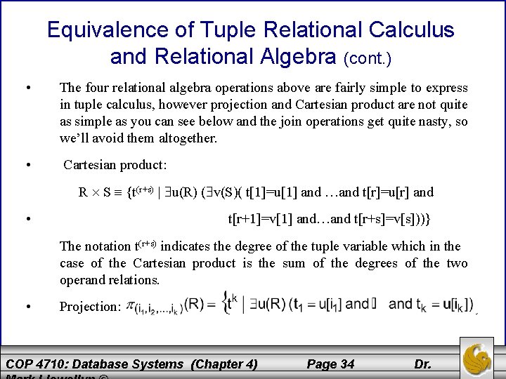
Equivalence of Tuple Relational Calculus and Relational Algebra (cont. ) • The four relational algebra operations above are fairly simple to express in tuple calculus, however projection and Cartesian product are not quite as simple as you can see below and the join operations get quite nasty, so we’ll avoid them altogether. • Cartesian product: R S {t(r+s) | u(R) ( v(S)( t[1]=u[1] and …and t[r]=u[r] and • t[r+1]=v[1] and…and t[r+s]=v[s]))} The notation t(r+s) indicates the degree of the tuple variable which in the case of the Cartesian product is the sum of the degrees of the two operand relations. • Projection: COP 4710: Database Systems (Chapter 4) Page 34 Dr.

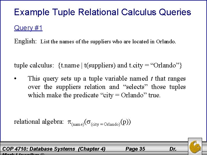
Example Tuple Relational Calculus Queries Query #1 English: List the names of the suppliers who are located in Orlando. tuple calculus: {t. name | t(suppliers) and t. city = “Orlando”} • This query sets up a tuple variable named t that ranges over the suppliers relation and “selects” those tuples which make the predicate “city = Orlando” true. relational algebra: (name)( (city = Orlando)(p)) COP 4710: Database Systems (Chapter 4) Page 35 Dr.

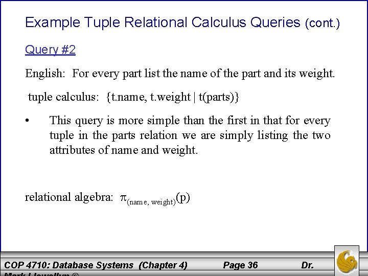
Example Tuple Relational Calculus Queries (cont. ) Query #2 English: For every part list the name of the part and its weight. tuple calculus: {t. name, t. weight | t(parts)} • This query is more simple than the first in that for every tuple in the parts relation we are simply listing the two attributes of name and weight. relational algebra: (name, weight)(p) COP 4710: Database Systems (Chapter 4) Page 36 Dr.

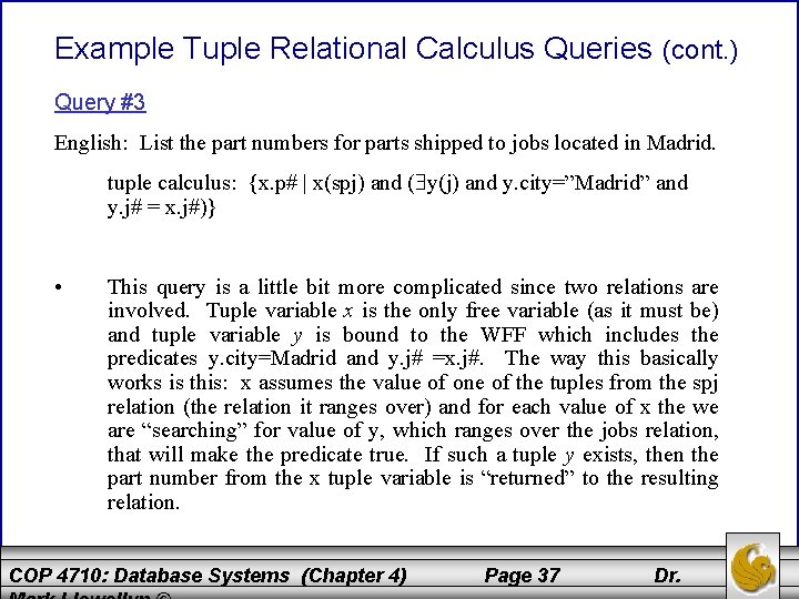
Example Tuple Relational Calculus Queries (cont. ) Query #3 English: List the part numbers for parts shipped to jobs located in Madrid. tuple calculus: {x. p# | x(spj) and ( y(j) and y. city=”Madrid” and y. j# = x. j#)} • This query is a little bit more complicated since two relations are involved. Tuple variable x is the only free variable (as it must be) and tuple variable y is bound to the WFF which includes the predicates y. city=Madrid and y. j# =x. j#. The way this basically works is this: x assumes the value of one of the tuples from the spj relation (the relation it ranges over) and for each value of x the we are “searching” for value of y, which ranges over the jobs relation, that will make the predicate true. If such a tuple y exists, then the part number from the x tuple variable is “returned” to the resulting relation. COP 4710: Database Systems (Chapter 4) Page 37 Dr.

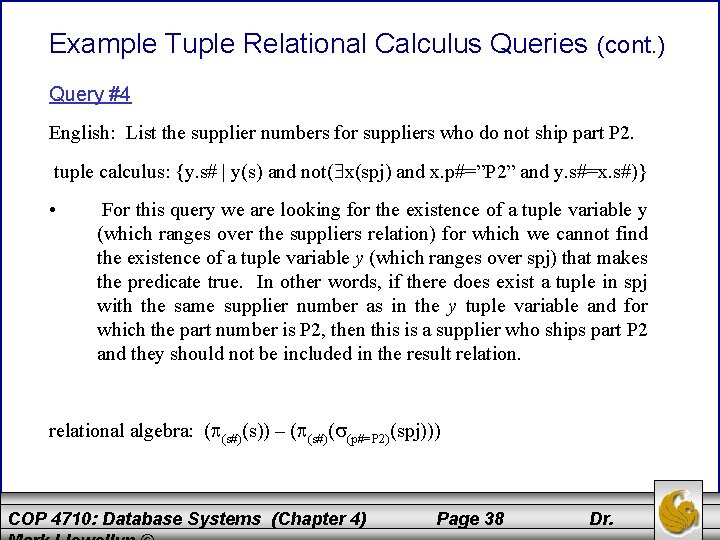
Example Tuple Relational Calculus Queries (cont. ) Query #4 English: List the supplier numbers for suppliers who do not ship part P 2. tuple calculus: {y. s# | y(s) and not( x(spj) and x. p#=”P 2” and y. s#=x. s#)} • For this query we are looking for the existence of a tuple variable y (which ranges over the suppliers relation) for which we cannot find the existence of a tuple variable y (which ranges over spj) that makes the predicate true. In other words, if there does exist a tuple in spj with the same supplier number as in the y tuple variable and for which the part number is P 2, then this is a supplier who ships part P 2 and they should not be included in the result relational algebra: ( (s#)(s)) – ( (s#)( (p#=P 2)(spj))) COP 4710: Database Systems (Chapter 4) Page 38 Dr.

Quantifier Implications and Equivalences • In general, the quantifiers can be transformed into the other quantifier with negation, and/or replace one another, a negated formula becomes un-negated an un-negated formula becomes negated. • There are however, some special cases which arise in these equivalences of which you need to be aware. • A few of the more important ones are shown below along with one which is commonly used by many people, but is incorrect! COP 4710: Database Systems (Chapter 4) Page 39 Dr.

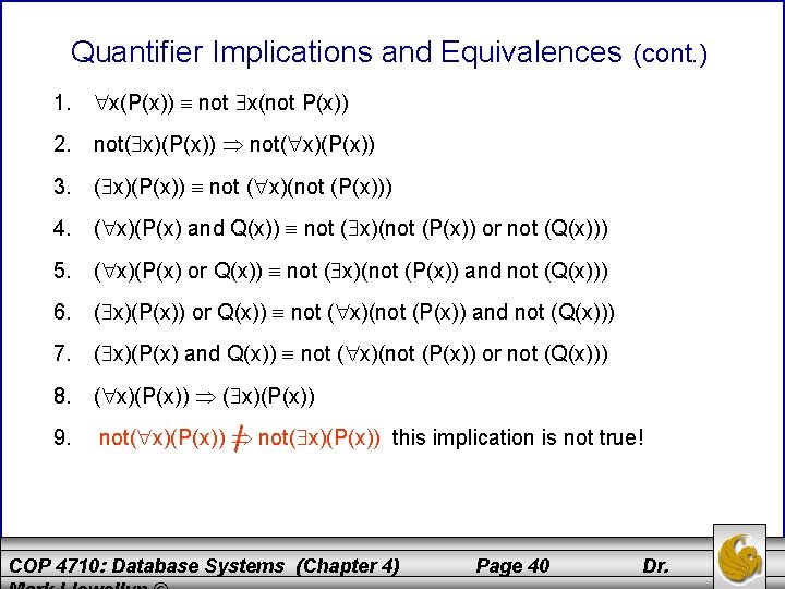
Quantifier Implications and Equivalences (cont. ) 1. x(P(x)) not x(not P(x)) 2. not( x)(P(x)) 3. ( x)(P(x)) not ( x)(not (P(x))) 4. ( x)(P(x) and Q(x)) not ( x)(not (P(x)) or not (Q(x))) 5. ( x)(P(x) or Q(x)) not ( x)(not (P(x)) and not (Q(x))) 6. ( x)(P(x)) or Q(x)) not ( x)(not (P(x)) and not (Q(x))) 7. ( x)(P(x) and Q(x)) not ( x)(not (P(x)) or not (Q(x))) 8. ( x)(P(x)) 9. not( x)(P(x)) this implication is not true! COP 4710: Database Systems (Chapter 4) Page 40 Dr.

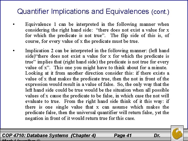
Quantifier Implications and Equivalences (cont. ) • Equivalence 1 can be interpreted in the following manner when considering the right hand side: “there does not exist a value for x for which the predicate is not true”. The flip side of this is, of course, for every value of x the predicate must be true. • Implication 2 can be interpreted in the following manner: (left hand side)“there does not exist a value for x for which the predicate is true” implies that (right hand side) the predicate is not true for every value of x”. This one you might have to think about for a minute. Looking at it from another direction consider this: if there exists a value of x that makes the predicate true, then the not in front of the expression would result in a value of false. So, the only way that the left hand side could be true would be the situation when all possible values of x cause the predicate to be false, in which case the not will evaluate to true. From the right hand side think of it this way: if there is one single value that x can assume which makes the predicate false, then the universal quantifier will return false, yet the negation in front of it would return true for this case. COP 4710: Database Systems (Chapter 4) Page 41 Dr.

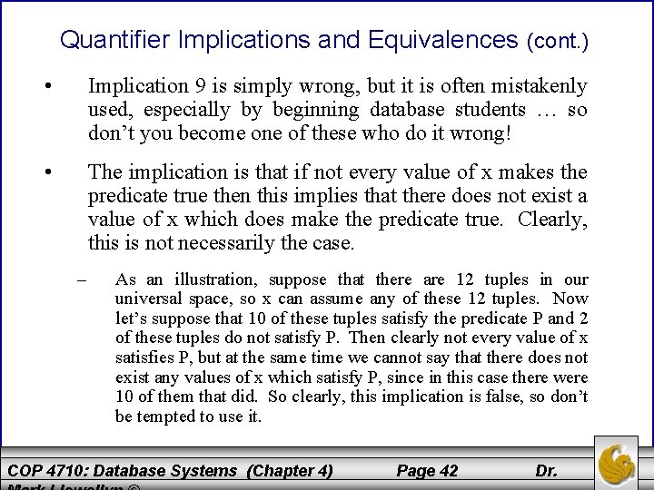
Quantifier Implications and Equivalences (cont. ) • Implication 9 is simply wrong, but it is often mistakenly used, especially by beginning database students … so don’t you become one of these who do it wrong! • The implication is that if not every value of x makes the predicate true then this implies that there does not exist a value of x which does make the predicate true. Clearly, this is not necessarily the case. – As an illustration, suppose that there are 12 tuples in our universal space, so x can assume any of these 12 tuples. Now let’s suppose that 10 of these tuples satisfy the predicate P and 2 of these tuples do not satisfy P. Then clearly not every value of x satisfies P, but at the same time we cannot say that there does not exist any values of x which satisfy P, since in this case there were 10 of them that did. So clearly, this implication is false, so don’t be tempted to use it. COP 4710: Database Systems (Chapter 4) Page 42 Dr.