Coordinate Transformations 2 D Coordinate Systems 2 D

Coordinate Transformations 2 D Coordinate Systems

2 D Coordinate Systems Before maps can be drawn, the positions, or co-ordinates, of the mapped points must all be in one single co-ordinate system. Thus if more than one co-ordinate systems are involved, they would need to be converted. To do that, one usually retains one co-ordinate system and converts all the positions which refer to all the other coordinate systems, to make them refer to the required system. This conversion is called a co-ordinate transformation.

2 D Coordinate Systems A 2 -D co-ordinate system consists of an origin, two axes that intersect at that origin and either one or two scale factors. Examples of 2 -D co-ordinate systems include: the UTM coordinate system, the co-ordinate systems on a digitizer, scanner and aerial photograph.

2 D Coordinate Systems ORIGIN For the two dimensional system, the origin is defined by specifying its two co-ordinates (X 0, Y 0) for example, one along the first axis and the other along the second axis. These two co-ordinates are arbitrary but they are often taken to be equal to zero. origins

2 D Coordinate Systems ORIENTATION If the two axes are at right angles to each other, the system is called an orthogonal co-ordinate system. In rare cases, the angle between them is something other than 90 degrees. In this case the system is called a non-orthogonal system. If the axes are orthogonal, then defining the orientation of one axis would automatically define that of the other. Therefore only one angle is needed to define the orientation of a 2 -D orthogonal co-ordinate system. If, however, the axes are non-orthogonal, then defining the orientation of one axis would not define the orientation of the other since the angle between them is unknown. Therefore two angles are needed to define the orientation of a 2 -D nonorthogonal co-ordinate system; the orientation of the first axis and the angle between the axes.

2 D Coordinate Systems orientation

2 D Coordinate Systems SCALE If a unit distance has the same length along the X as well as the Y axis, we say that the co-ordinate system has a homogeneous scale. In that case, knowing the distance of one line defines the scale of the system uniquely, no matter in which direction that distance extends. If, however, a unit length along the X axis is different from a unit length along the Y axis, then the 2 -D system possesses two scale factors; Sx and Sy for example.

2 D Coordinate Systems The possible permutations for the definition of the 2 -D co-ordinate system are therefore TYPE OF 2 -D SYSTEM NUMBER OF PARAMETERS REQUIRED SYSTEM ORIGIN ORIENTATION SCALE 2 -d non-orthogonal non-homogeneous scale 2 2 -d non-orthogonal homogeneous scale 2 -d orthogonal non-homogeneous scale 2 -d orthogonal homogeneous scale 2 2 1 1

2 D Coordinate Systems DEFINING THE PARAMETERS ORIGIN The origin is usually arbitrarily defined. For example, the origin of a digitiser or a scanner is taken to be in one of its four corners and that of an aerial photograph system is usually at the intersection of the tic marks.

2 D Coordinate Systems ORIENTATION The orientation may be either arbitrary or physically meaningful, A chain line and offsets is an example of an arbitrary orientation in a co-ordinate system. In this situation, the surveyor chooses one line, usually a boundary line to be an axis of the system and then defines the other axis as being orthogonal to it. A physically meaningful choice of orientation may be the axis of a digitiser or a scanner co-ordinate system being parallel to its two edges. The axes of the UTM system are also attached in some way to the actual north-south direction on the Earth surface.

2 D Coordinate Systems SCALE The scale factor must be defined or may be determined by computing from known distances on the projection and the corresponding distances on the ground.

2 -D Conformal Coordinate Transformation 2 -D CONFORMAL TRANSFORMATION A 2 -D conformal transformation is a scale homogeneous, orthogonal transformation requiring 4 parameters – 1 scale, 1 orientation, 2 translations Consider a line AB on 2 superimposed coordinate systems The coordinates of the points A and B are known on both systems EB NB R A B Coordinate system 2 Coordinate system 1

2 -D Conformal Coordinate Transformation The scale or units of measurement on the 2 systems are different. To transform from system 1 to system 2 the scale must be found The scaled coordinates of the points in coordinate system 1 to coordinate system 2 are: Any point on system 1 can be scaled to system 2

2 -D Conformal Coordinate Transformation The orientation of the 2 systems are different EB NB Consider point B θ R A B Coordinate system 2 Coordinate system 1

2 -D Conformal Coordinate Transformation On coordinate system 2 the same point B EB α θ R A B NB Coordinate system 2 Coordinate system 1

2 -D Conformal Coordinate Transformation Expanding using sum of sines and cosines since

2 -D Conformal Coordinate Transformation The angles θ and α can be found by

2 -D Conformal Coordinate Transformation A translation is required since the origin of the 2 systems are different Consider the situation where the origins are shifted B X 0, Y 0 (TE, TN) (0, 0) Coordinate system 1 Coordinate system 2

2 -D AFFINE TRANSFORMATION Unique and Least Squares Solutions

2 -D Affine Transformation 2 -D Conformal transformations include 2 parameters for change in origin (or translation), 1 parameter for change in orientation and 1 parameter for change in scale. 2 -D affine transformations include 2 parameters for change in origin, 2 parameters for change in scale and 2 parameters for change in orientation. The form of the 2 -D conformal transformation equations was reduced to: The form of the 2 -D affine transformation equations is reduced to the form:

2 -D Affine Transformation The usual application of the 2 -D affine transformation equations (as it was with the 2 -D conformal equations) is when the parameters are first determined by utilizing known co-located points and then the equations with the known parameters included are applied to points known on one system to transform them to the other system. Three co-located points are required from which 6 equations can be derived in order to determine the 6 parameters uniquely

2 -D Affine Transformation For 3 co-located points, the equations are:

2 -D Affine Transformation These equations are of the linear equation form: n 1 1 m. A n. X = m. L Where there are m equations and n unknowns and m = n so that:

2 -D Affine Transformation The parameters can therefore be determined using matrix methods: And other points may be transformed using matrix methods:

2 -D Affine Transformation When there is redundant information or more than 3 points are known on both systems, least squares may be used. For example if 4 points are known on both systems: 1) From the measurement equations:

2 -D Affine Transformation 2) Form the observation equations:

2 -D Affine Transformation 3) Square the residuals and sum:

2 -D Affine Transformation 4) Take partial differentials with respect to each unknown and equate to zero: Normal equations 5) Solve simultaneously to obtain unique values for the unknowns

2 -D Affine Transformation It was shown previously that the normal equations can be formed directly using matrix methods:

2 -D Affine Transformation Example Wolf and Dewitt (2000) Point Comparator coord x mm Comparator coord y mm Calibrated coords X mm Calibrated coords Y mm Fiducial A 228. 170 129. 730 112. 995 0. 034 Fiducial B 2. 100 129. 520 -113. 006 0. 005 Fiducial C 115. 005 242. 625 0. 003 112. 993 Fiducial D 115. 274 16. 574 -0. 012 -113. 000 1 206. 674 123. 794 2 198. 365 132. 856 3 91. 505 18. 956

2 -D Affine Transformation

2 -D Affine Transformation AX = L

2 -D Affine Transformation

Conformal Coordinate Transformations Conformal Transformation Example

Conformal Transformation Example Four parameter co-ordinate transformation The co-ordinates of two points A and B are listed in Table 1 for two separate co-ordinate systems e-n (an outdated system) and E-N (the revised system). A point C has co-ordinates on the old system of e = 15, 362. 88 ft. and n = 14622. 70 ft. • i) calculate the co-ordinates of point C on the E-N system POINT e (ft. ) n (ft) E (m) N (m) A 16, 719. 24 12, 164. 51 538, 712. 09 203, 683. 60 B 18, 975. 69 13, 192. 83 539, 151. 00 204, 298. 92

Conformal Transformation Example SCALE = 0. 30479 or 0. 3048 (the factor used to convert feet to meters)

Conformal Transformation Example

Conformal Transformation Example ROTATION θ A System 2 α System 1

Conformal Transformation Example

Conformal Transformation Example TRANSLATION

Conformal Transformation Example Now that the parameters are known, other coordinated points such as point C can be transformed: e = 15, 362. 88 ft. and n = 14622. 70 ft. C scaled coords:

Conformal Transformation Example C rotated coords:

Conformal Transformation Example C translated coords:

2 -D Conformal Coordinate Transformations Computerized Methods

Computerized Methods in Transformations To computerize the transformation process the equations must be standardized and combined: Moving from system 1 to system 2 the scale equations are substituted into the rotation equations:

Computerized Methods in Transformations The angle is standardized as system 1 -system 2 and the translation parameters are added on to complete the transformation equations:

Computerized Methods in Transformations Now substitute: To get:

Computerized Methods in Transformations The scale and rotation need not be determined but if need be:

Computerized Methods in Transformations - example From the previous example:

Computerized Methods in Transformations - example Solving simultaneously: Substituting:

Computerized Methods in Transformations - example The equations may be expressed as matrices: For each pair of equations

Computerized Methods in Transformations - example or For each pair of equations 2 x 1 2 x 2 2 x 1

Computerized Methods in Transformations - example The individual equations can also be put into the matrix format for solution via inversion: AX = L So that: X = A-1 L X or the unknowns can be solved using a spreadsheet and then the parameters can be applied to other points to be transformed

Computerized Methods in Transformations – example Using the previous example

Least Squares in Transformations Introduction

Least Squares in Transformations The observation equation method of Least Squares may be used in the computation of the transformation parameters More than 2 co-located points (points coordinated on both systems) must be known to perform Least Squares minimizes the sum of the squares of the residuals resulting in the best estimate of the value of the unknowns

Least Squares in Transformations Simple example of least squares method (Wolf and Dewitt 2000) Given the following measurement equations x+y=3. 0 x=1. 5 y=1. 4 m = number of observations = 3 n=number of unknowns = (x and y) = 2 Solving equations (1) and (2) gives x = 1. 5 and y =1. 5 Solving equations (2) and (3) gives x = 1. 5 and y = 1. 4 Solving equations (1) and (3) gives x = 1. 6 and y = 1. 4

Least Squares in Transformations The measurements therefore contain errors so these can be included in the equations Observation equations There are many values that the residuals may take so that the same values are obtained for x and y no matter which equations are used to solve for them For example: or

Least Squares in Transformations However the values of the residuals which minimize the sum of the square of the residuals are the most probable values for the residuals. To obtain these values the following procedure is adopted 1) Square the residuals

Least Squares in Transformations 2) Sum the squared residuals together 3) Minimize the sum of the square of the residuals by taking partial derivatives with respect to each unknown and setting them equal to zero Normal Equations

Least Squares in Transformations The simplified normal equations are: There are now the same number of normal equations as there are unknowns leading to a unique solution for the unknowns when solved

Least Squares in Transformations These values may be plugged back into the observation equations to determine the residuals The sum of the squares of the residuals for the example solutions may be compared with the sum of the squares of the residuals derived by the least squares method

Least Squares in Transformations The process forming normal equations is lengthy and time consuming but a systematic procedure can be performed If there are m observation equations in n unknowns:

Least Squares in Transformations The residuals are squared and summed Partial derivatives are taken with respect to each unknown n normal equations are formed Simplifying the normal equations by reducing and factoring results in the standardized format as follows:

Least Squares in Transformations The coefficients may be computed and set up in a table to facilitate the construction of the normal equations Example from the previous problem Observation equations A=3 x 2 X=2 x 1 L=3 x 1 V=3 x 1

Least Squares in Transformations Equation number (i) 1 1 1 3. 0 2 1 0 1. 5 1 0 0 1. 5 0. 0 3 0 1 1. 4 0 0 1 0. 0 1. 4

Least Squares in Transformations The normal equations in the standardized format are therefore: Substituting from the table gives: The normal equations may now be solved to determine the unknowns

Least Squares in Transformations The matrix method proves to be simpler for solving the equations The observation equations are represented generally as: The normal equations as obtained in the standardized method are equivalent to: So that AT A is the matrix of normal equation coefficients of the unknowns

Least Squares in Transformations Premultiply both sides by the inverse of the AT A matrix to result in: Reducing : The unknowns can then be simply determined

Least Squares in Transformations Example from previous problem: Observation equations

Least Squares in Transformations

Least Squares in Transformations

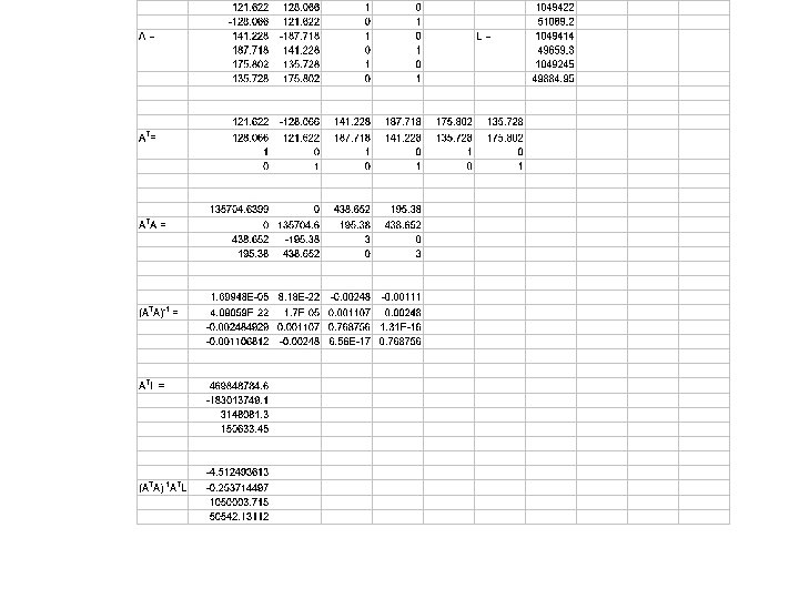
Least Squares in Transformations The Least Squares method applied to the general 2 -D conformal coordinate transformation For each co-located point of m observed points two equations are obtained The unknowns are a, b, TE and TN

Least Squares in Transformations Observation equations can be formed Which are of the form: A is the matrix of coefficients of the unknown transformation parameters or the coordinates on one system, X is the matrix of the unknown transformation parameters, L is the matrix of observations which are the control coordinates and V is the matrix of residuals or measurement errors

Least Squares in Transformations

Least Squares in Transformations We can go directly to the normal equations to solve for the unknowns knowing that the normal equations are simply: Therefore:

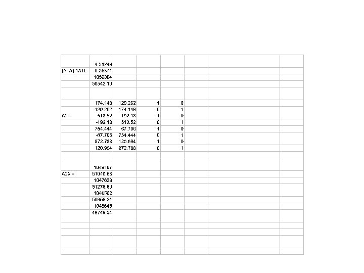
Least Squares in Transformations – example (Wolf and Ghilani 1997) Given the co-located points A, B and C, find the best estimate of the transformation parameters and then transform points 1, 2, 3 and 4 Point Easting Northing A 1049422. 40 51089. 20 B 1049413. 95 49659. 30 C 1049244. 95 49884. 95 1 2 3 4 X 121. 622 141. 228 175. 802 174. 148 513. 520 754. 444 972. 788 Y -128. 066 187. 718 135. 728 -120. 262 -192. 130 -67. 706 120. 994