Convolutional Neural Networks for CAP 4453 Recap From

Convolutional Neural Networks for CAP 4453

Recap From previous lecture: ● Neural Networks receive an input (a single vector), and transform it through a series of hidden layers. ● Each hidden layer is made up of a set of neurons, where each neuron is fully connected to all neurons in the previous layer. ● Neurons in a single layer function completely independently and do not share any connections. ● The last fully-connected layer is called the “output layer”

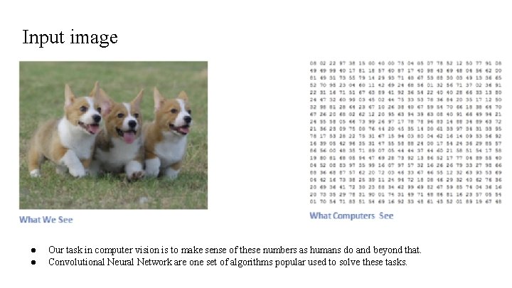
Input image ● ● Our task in computer vision is to make sense of these numbers as humans do and beyond that. Convolutional Neural Network are one set of algorithms popular used to solve these tasks.

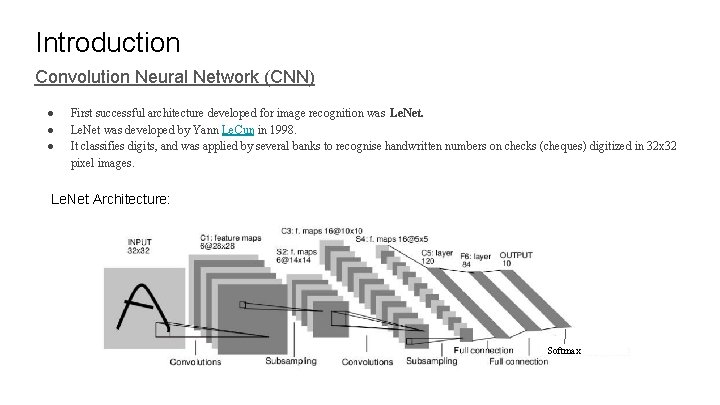
Introduction Convolution Neural Network (CNN) ● ● ● First successful architecture developed for image recognition was Le. Net was developed by Yann Le. Cun in 1998. It classifies digits, and was applied by several banks to recognise handwritten numbers on checks (cheques) digitized in 32 x 32 pixel images. Le. Net Architecture: Softmax

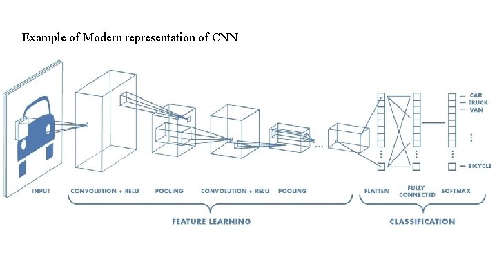
Example of Modern representation of CNN

Introduction to CNN ● ● ● Core building block of CNN is called Convolutional layer (Conv layer). Convolutional layer perform convolution operations. These operations are performed using set of filters. These filters are learnable parameters for the network. Every filter is small matrix that extends through the full depth of the input volume. These filter parameters extract complex features from your data.

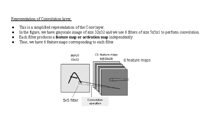
Representation of Convolution layer: ● ● This is a simplified representation of the Conv layer. In the figure, we have grayscale image of size 32 x 32 and we use 6 filters of size 5 x 5 x 1 to perform convolution. Each filter produces a feature map or activation map independently. Thus, we have 6 feature maps corresponding to each filter. 6 feature maps 5 x 5 filter Convolution operation

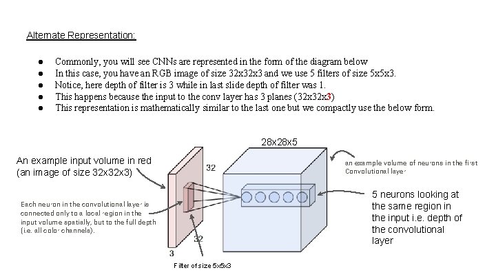
Alternate Representation: ● ● ● Commonly, you will see CNNs are represented in the form of the diagram below In this case, you have an RGB image of size 32 x 3 and we use 5 filters of size 5 x 5 x 3. Notice, here depth of filter is 3 while in last slide depth of filter was 1. This happens because the input to the conv layer has 3 planes (32 x 3) This representation is mathematically similar to the last one but we compactly use the below form. 28 x 5 An example input volume in red (an image of size 32 x 3) an example volume of neurons in the first Convolutional layer 5 neurons looking at the same region in the input i. e. depth of the convolutional layer Each neuron in the convolutional layer is connected only to a local region in the input volume spatially, but to the full depth (i. e. all color channels). Filter of size 5 x 5 x 3

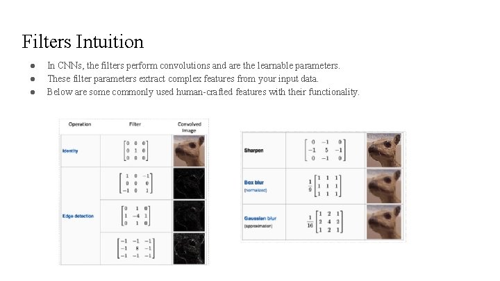
Filters Intuition ● ● ● In CNNs, the filters perform convolutions and are the learnable parameters. These filter parameters extract complex features from your input data. Below are some commonly used human-crafted features with their functionality.

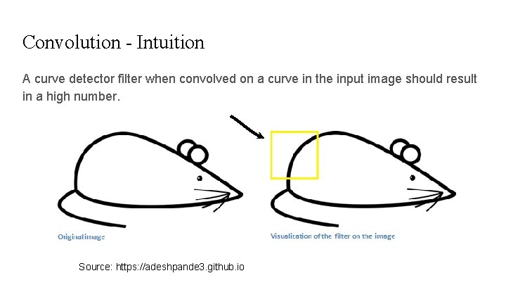
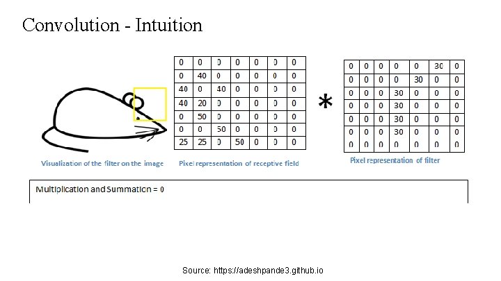
Convolution - Intuition A curve detector filter when convolved on a curve in the input image should result in a high number. Source: https: //adeshpande 3. github. io

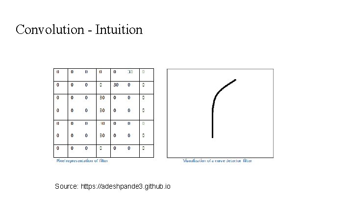
Convolution - Intuition Source: https: //adeshpande 3. github. io

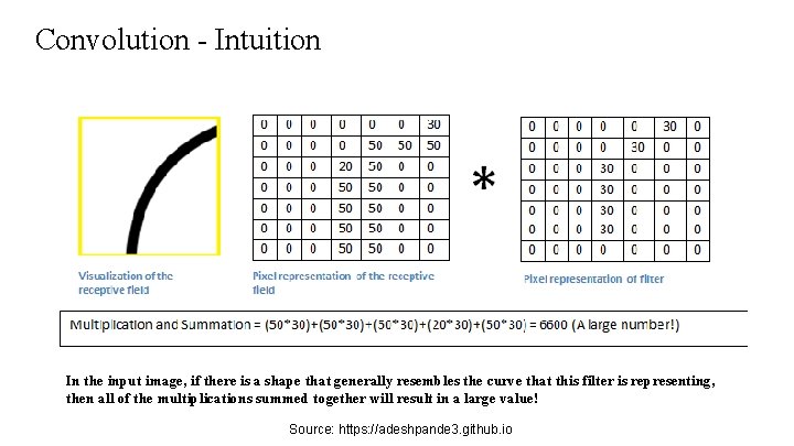
Convolution - Intuition In the input image, if there is a shape that generally resembles the curve that this filter is representing, then all of the multiplications summed together will result in a large value! Source: https: //adeshpande 3. github. io

Convolution - Intuition Source: https: //adeshpande 3. github. io

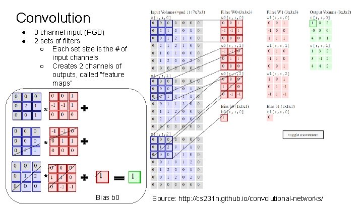
Convolution ● ● 3 channel input (RGB) 2 sets of filters ○ Each set size is the # of input channels ○ Creates 2 channels of outputs, called “feature maps” * * * Bias b 0 Source: http: //cs 231 n. github. io/convolutional-networks/

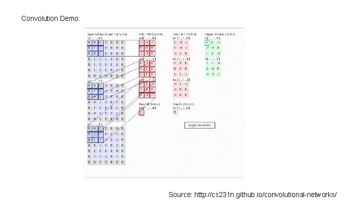
Convolution Demo: Source: http: //cs 231 n. github. io/convolutional-networks/

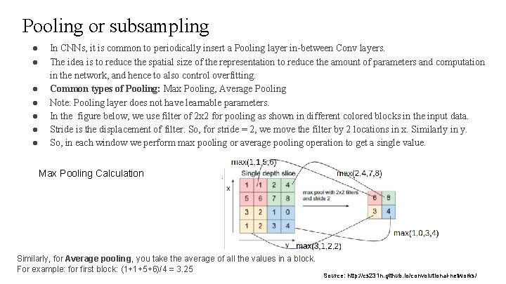
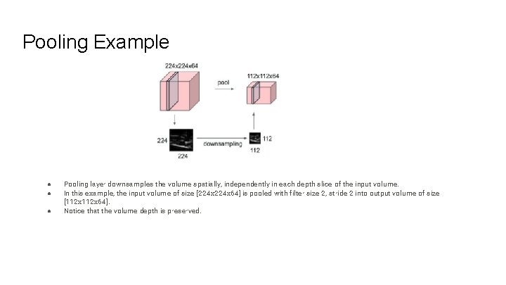
Pooling or subsampling ● ● ● ● In CNNs, it is common to periodically insert a Pooling layer in-between Conv layers. The idea is to reduce the spatial size of the representation to reduce the amount of parameters and computation in the network, and hence to also control overfitting. Common types of Pooling: Max Pooling, Average Pooling Note: Pooling layer does not have learnable parameters. In the figure below, we use filter of 2 x 2 for pooling as shown in different colored blocks in the input data. Stride is the displacement of filter. So, for stride = 2, we move the filter by 2 locations in x. Similarly in y. So, in each window we perform max pooling or average pooling operation to get a single value. Max Pooling Calculation Similarly, for Average pooling, you take the average of all the values in a block. For example: for first block: (1+1+5+6)/4 = 3. 25 Source: http: //cs 231 n. github. io/convolutional-networks/

Pooling Example ● ● ● Pooling layer downsamples the volume spatially, independently in each depth slice of the input volume. In this example, the input volume of size [224 x 64] is pooled with filter size 2, stride 2 into output volume of size [112 x 64]. Notice that the volume depth is preserved.

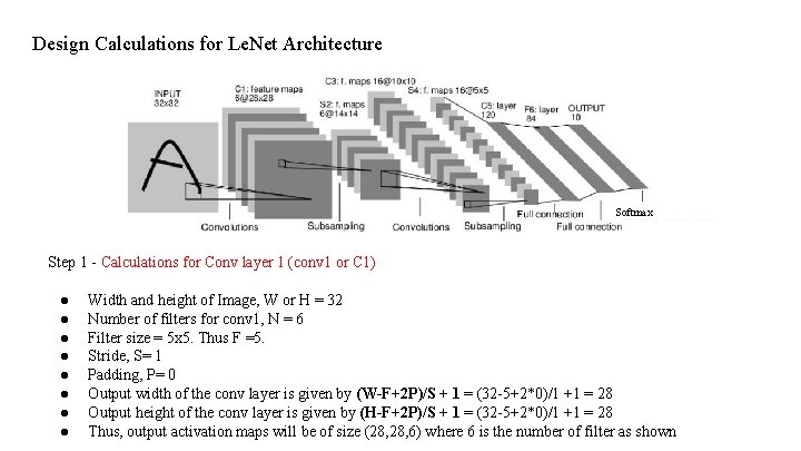
Design Calculations for Le. Net Architecture Softmax Step 1 - Calculations for Conv layer 1 (conv 1 or C 1) ● ● ● ● Width and height of Image, W or H = 32 Number of filters for conv 1, N = 6 Filter size = 5 x 5. Thus F =5. Stride, S= 1 Padding, P= 0 Output width of the conv layer is given by (W-F+2 P)/S + 1 = (32 -5+2*0)/1 +1 = 28 Output height of the conv layer is given by (H-F+2 P)/S + 1 = (32 -5+2*0)/1 +1 = 28 Thus, output activation maps will be of size (28, 6) where 6 is the number of filter as shown

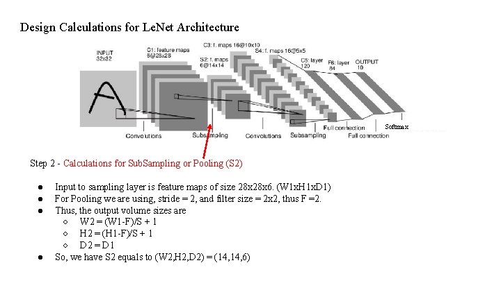
Design Calculations for Le. Net Architecture Softmax Step 2 - Calculations for Sub. Sampling or Pooling (S 2) ● ● Input to sampling layer is feature maps of size 28 x 6. (W 1 x. H 1 x. D 1) For Pooling we are using, stride = 2, and filter size = 2 x 2, thus F =2. Thus, the output volume sizes are ○ W 2 = (W 1 -F)/S + 1 ○ H 2 = (H 1 -F)/S + 1 ○ D 2 = D 1 So, we have S 2 equals to (W 2, H 2, D 2) = (14, 6)

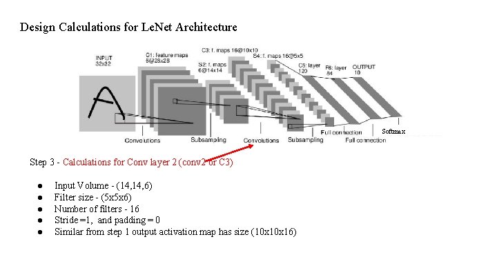
Design Calculations for Le. Net Architecture Softmax Step 3 - Calculations for Conv layer 2 (conv 2 or C 3) ● ● ● Input Volume - (14, 6) Filter size - (5 x 5 x 6) Number of filters - 16 Stride =1, and padding = 0 Similar from step 1 output activation map has size (10 x 16)

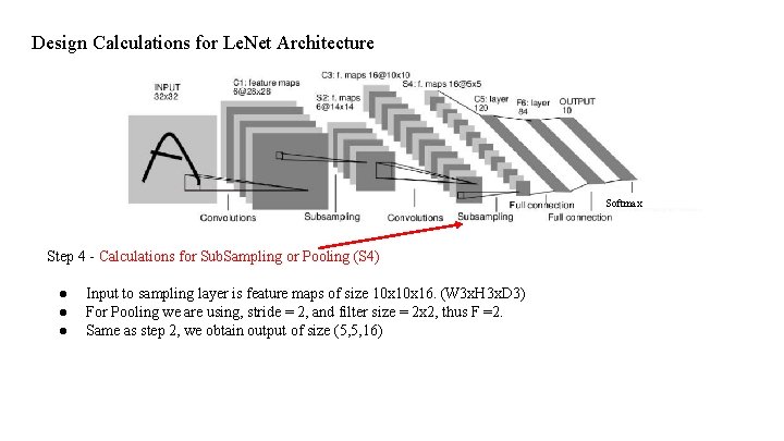
Design Calculations for Le. Net Architecture Softmax Step 4 - Calculations for Sub. Sampling or Pooling (S 4) ● ● ● Input to sampling layer is feature maps of size 10 x 16. (W 3 x. H 3 x. D 3) For Pooling we are using, stride = 2, and filter size = 2 x 2, thus F =2. Same as step 2, we obtain output of size (5, 5, 16)

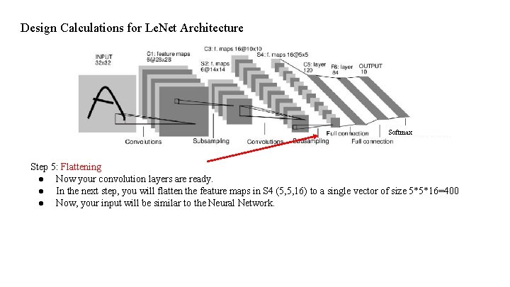
Design Calculations for Le. Net Architecture Softmax Step 5: Flattening ● Now your convolution layers are ready. ● In the next step, you will flatten the feature maps in S 4 (5, 5, 16) to a single vector of size 5*5*16=400 ● Now, your input will be similar to the Neural Network.

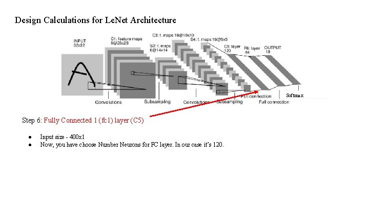
Design Calculations for Le. Net Architecture Softmax Step 6: Fully Connected 1 (fc 1) layer (C 5) ● ● Input size - 400 x 1 Now, you have choose Number Neurons for FC layer. In our case it’s 120.

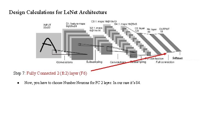
Design Calculations for Le. Net Architecture Softmax Step 7: Fully Connected 2 (fc 2) layer (F 6) ● Now, you have to choose Number Neurons for FC 2 layer. In our case it’s 84.

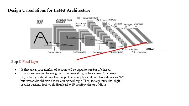
Design Calculations for Le. Net Architecture Softmax Step 8: Final layer ● ● In this layer, your number of neuron will be equal to number of classes. In our case, we will be using the 10 numerical digits, hence need 10 classes. So, in fact you should see that the picture example should not have shown an “A”, but instead should have shown a numerical digit. Thus, for any numerical digit used in training, that would then lead to 10 possible classes of digits.

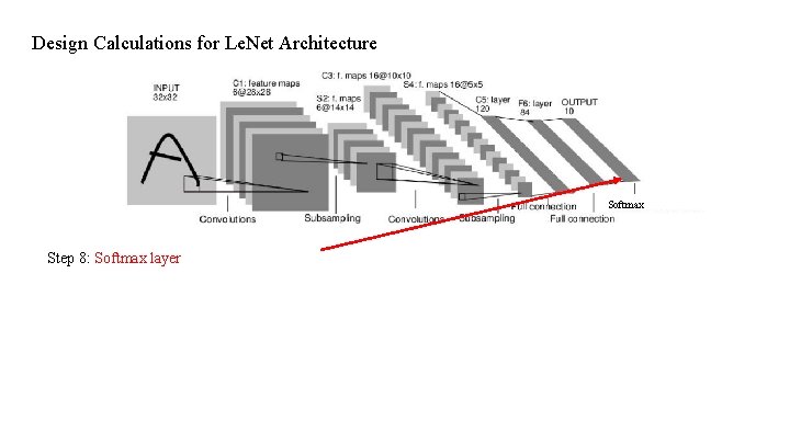
Design Calculations for Le. Net Architecture Softmax Step 8: Softmax layer

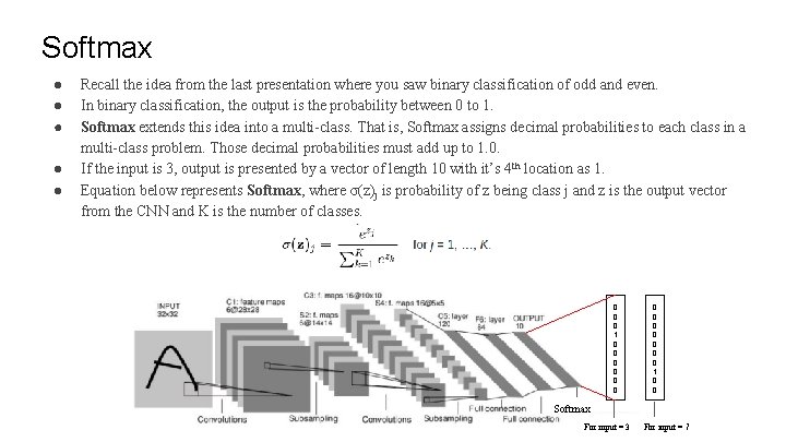
Softmax ● ● ● Recall the idea from the last presentation where you saw binary classification of odd and even. In binary classification, the output is the probability between 0 to 1. Softmax extends this idea into a multi-class. That is, Softmax assigns decimal probabilities to each class in a multi-class problem. Those decimal probabilities must add up to 1. 0. If the input is 3, output is presented by a vector of length 10 with it’s 4 th location as 1. Equation below represents Softmax, where σ(z)j is probability of z being class j and z is the output vector from the CNN and K is the number of classes. 0 0 0 1 0 0 0 0 1 0 0 Softmax For input = 3 For input = 7

Convolution + Re. LU ● ● From the slide 5, you can see that in convolution networks after conv layer we add a Re. LU or activation layer. Re. LU is added to introduce a non-linearity in the convolutional layer. (You have previously seen sigmoid. ) Introducing this nonlinearity gives CNNs the power to capture non-linear patterns in your data. Re. LU is a commonly used activation function in practice but there are other activations such as sigmoid, tanh etc. as mentioned in the Neural Network lecture earlier.

Summary ● ● ● CNNs are compact representation of Neural networks used for image understanding. CNNs are built using set of conv layers, pooling layers, activations functions, and fully connected layers connected in a specific manner. Conv layer has filters which are the learnable parameters of the network, while pooling layer has not parameters and lastly, fully connected layers parameters are same as Neural Network parameters. Softmax is often used for Multi-classification. The training procedure for CNN is same as that of Neural network but your data is in the form of 2 -D (generally images).