Convolutional Neural Network 20151002 Outline Neural Networks Convolutional

Convolutional Neural Network 2015/10/02 陳柏任

Outline • Neural Networks • Convolutional Neural Networks • Some famous CNN structure • Applications • Toolkit • Conclusion • Reference 2

Outline • Neural Networks • Convolutional Neural Networks • Some famous CNN structure • Applications • Toolkit • Conclusion • Reference 3

Our brain [1] 4

Neuron [2] 5

Neuron [2] 6

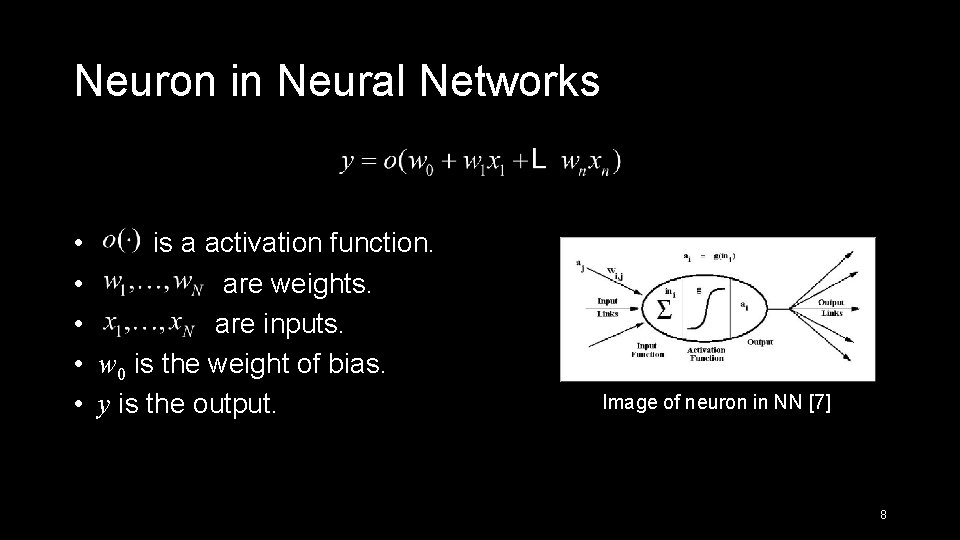
Bias Neuron Activation function Inputs Output Neuron in Neural Networks [3] 7

Neuron in Neural Networks • is a activation function. • are weights. • are inputs. • w 0 is the weight of bias. • y is the output. Image of neuron in NN [7] 8

Difference Between Biology and Engineering • Activation function • Bias 9

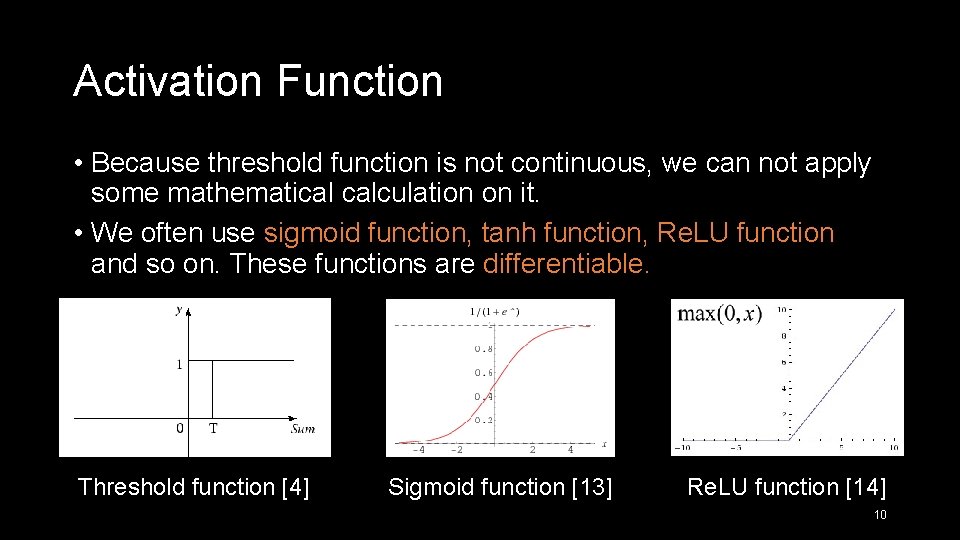
Activation Function • Because threshold function is not continuous, we can not apply some mathematical calculation on it. • We often use sigmoid function, tanh function, Re. LU function and so on. These functions are differentiable. Threshold function [4] Sigmoid function [13] Re. LU function [14] 10

Why should we need to add the bias term? 11

Without Bias Term [5] 12

With Bias Term [5] 13

Neural Networks (NNs) • Proposed in 1950 s • NNs are a family of machine learning models. 14

Neural Networks [6] 15

Neural Networks • Feed forward (No recurrences) • Fully-connected between layers • No connections between neurons in the layer 16

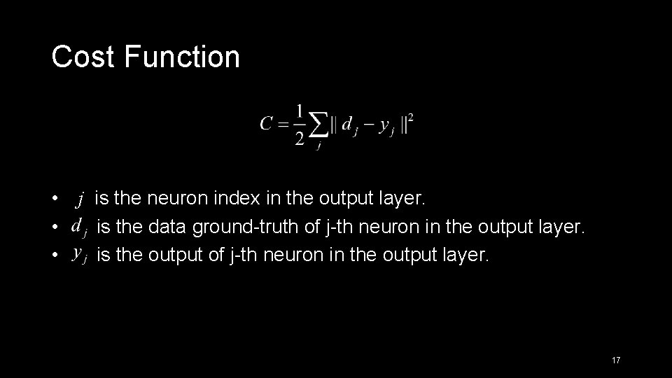
Cost Function • j is the neuron index in the output layer. • is the data ground-truth of j-th neuron in the output layer. • is the output of j-th neuron in the output layer. 17

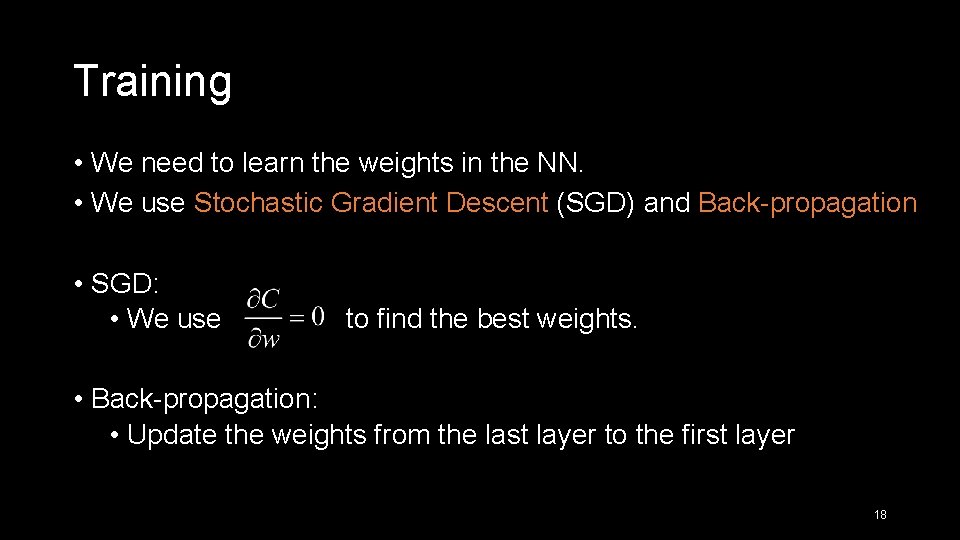
Training • We need to learn the weights in the NN. • We use Stochastic Gradient Descent (SGD) and Back-propagation • SGD: • We use to find the best weights. • Back-propagation: • Update the weights from the last layer to the first layer 18

Outline • Neural Networks • Convolutional Neural Networks • Some famous CNN structure • Applications • Toolkit • Conclusion • Reference 19

Neural Networks [6] Recall: Neural Networks 20

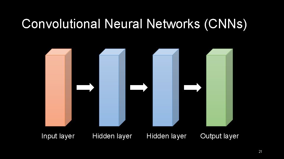
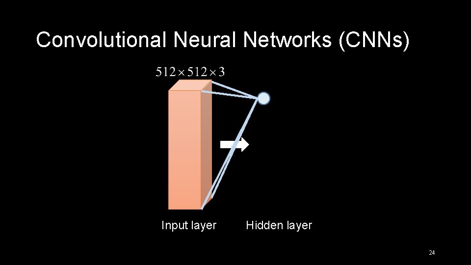
Convolutional Neural Networks (CNNs) Input layer Hidden layer Output layer 21

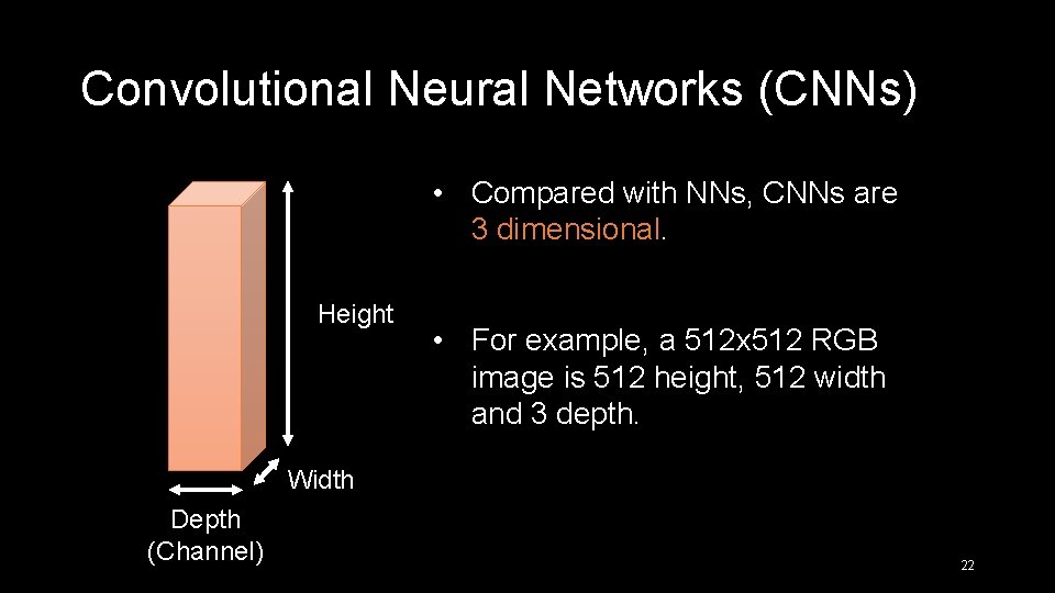
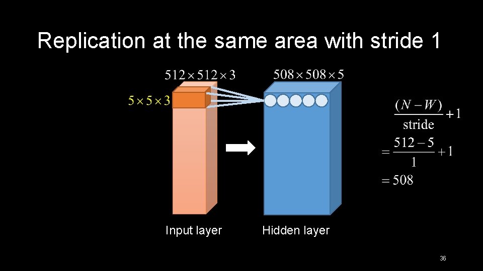
Convolutional Neural Networks (CNNs) • Compared with NNs, CNNs are 3 dimensional. Height • For example, a 512 x 512 RGB image is 512 height, 512 width and 3 depth. Width Depth (Channel) 22

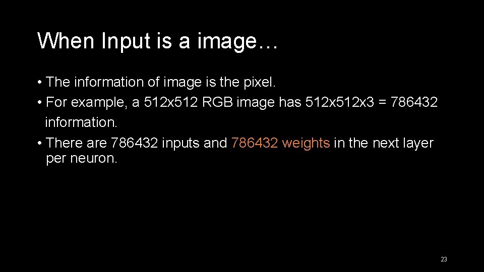
When Input is a image… • The information of image is the pixel. • For example, a 512 x 512 RGB image has 512 x 3 = 786432 information. • There are 786432 inputs and 786432 weights in the next layer per neuron. 23

Convolutional Neural Networks (CNNs) Input layer Hidden layer 24

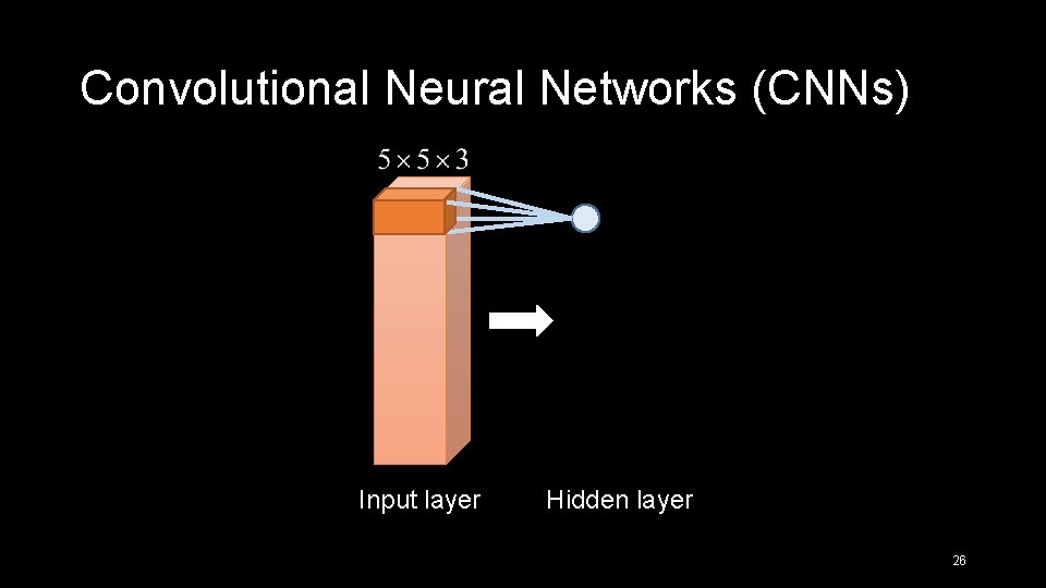
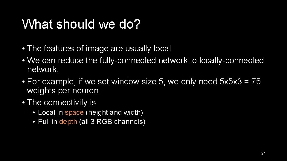
What should we do? • The features of image are usually local. • We can reduce the fully-connected network to locally-connected network. • For example, if we set window size 5 … 25

Convolutional Neural Networks (CNNs) Input layer Hidden layer 26

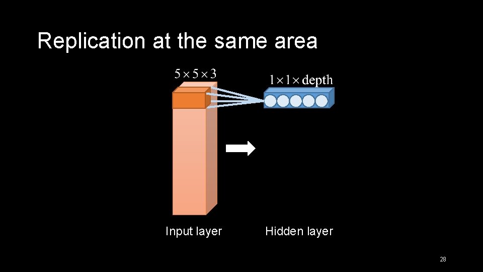
What should we do? • The features of image are usually local. • We can reduce the fully-connected network to locally-connected network. • For example, if we set window size 5, we only need 5 x 5 x 3 = 75 weights per neuron. • The connectivity is • Local in space (height and width) • Full in depth (all 3 RGB channels) 27

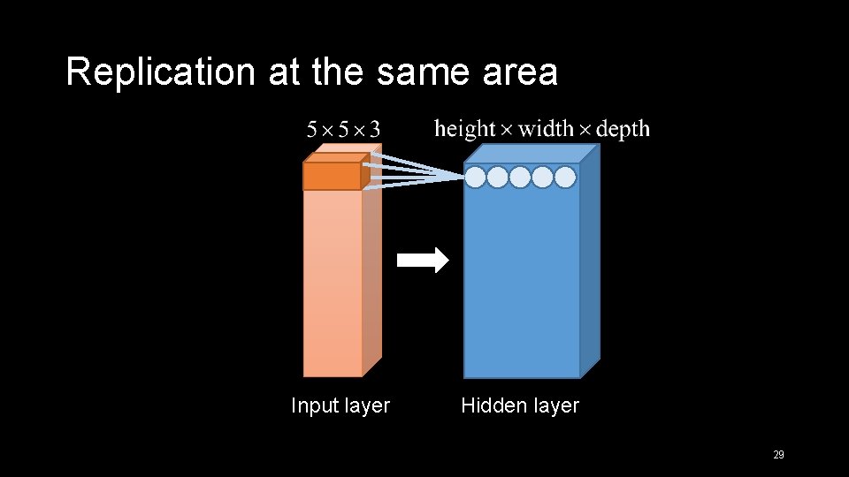
Replication at the same area Input layer Hidden layer 28

Replication at the same area Input layer Hidden layer 29

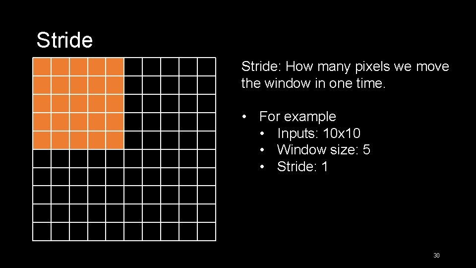
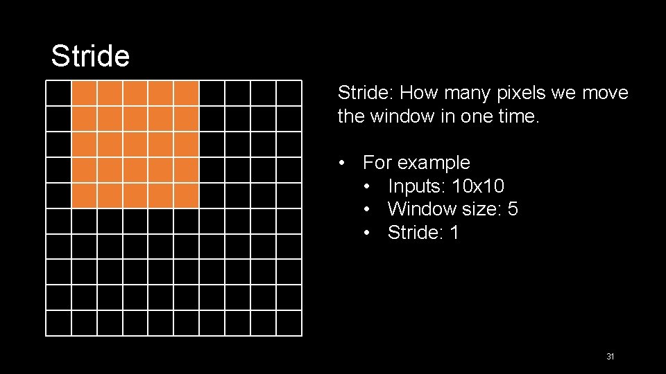
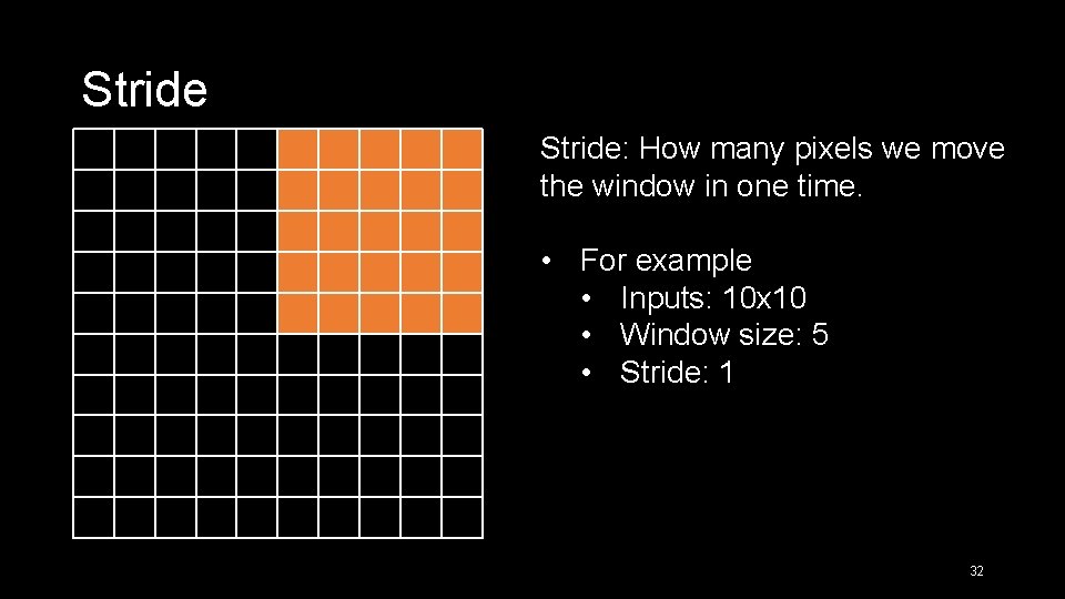
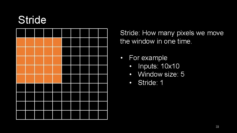
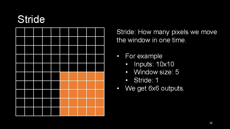
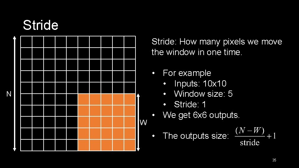
Stride: How many pixels we move the window in one time. • For example • Inputs: 10 x 10 • Window size: 5 • Stride: 1 30

Stride: How many pixels we move the window in one time. • For example • Inputs: 10 x 10 • Window size: 5 • Stride: 1 31

Stride: How many pixels we move the window in one time. • For example • Inputs: 10 x 10 • Window size: 5 • Stride: 1 32

Stride: How many pixels we move the window in one time. • For example • Inputs: 10 x 10 • Window size: 5 • Stride: 1 33

Stride: How many pixels we move the window in one time. • For example • Inputs: 10 x 10 • Window size: 5 • Stride: 1 • We get 6 x 6 outputs. 34

Stride: How many pixels we move the window in one time. N W • For example • Inputs: 10 x 10 • Window size: 5 • Stride: 1 • We get 6 x 6 outputs. • The outputs size: 35

Replication at the same area with stride 1 Input layer Hidden layer 36

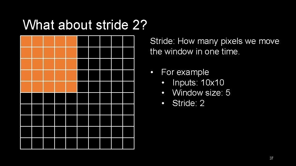
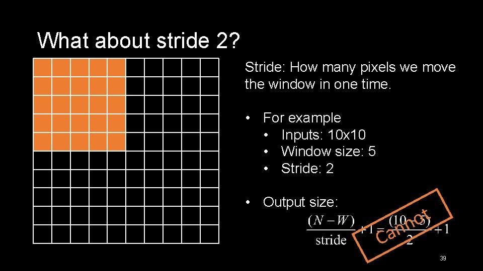
What about stride 2? Stride: How many pixels we move the window in one time. • For example • Inputs: 10 x 10 • Window size: 5 • Stride: 2 37

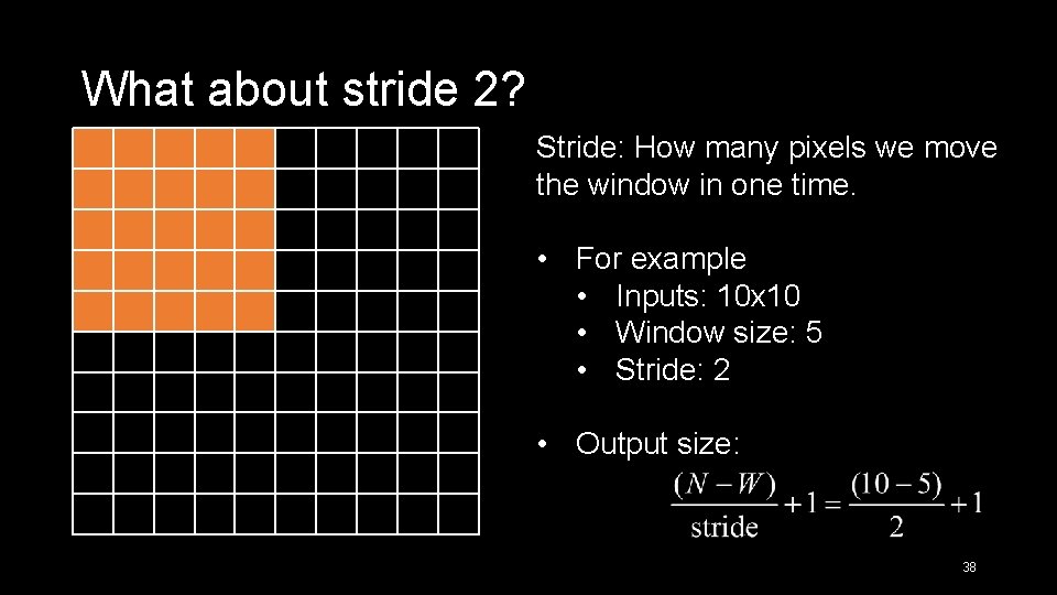
What about stride 2? Stride: How many pixels we move the window in one time. • For example • Inputs: 10 x 10 • Window size: 5 • Stride: 2 • Output size: 38

What about stride 2? Stride: How many pixels we move the window in one time. • For example • Inputs: 10 x 10 • Window size: 5 • Stride: 2 • Output size: t o nn Ca 39

There are some problem in stride … • The output size is smaller than input size. 40

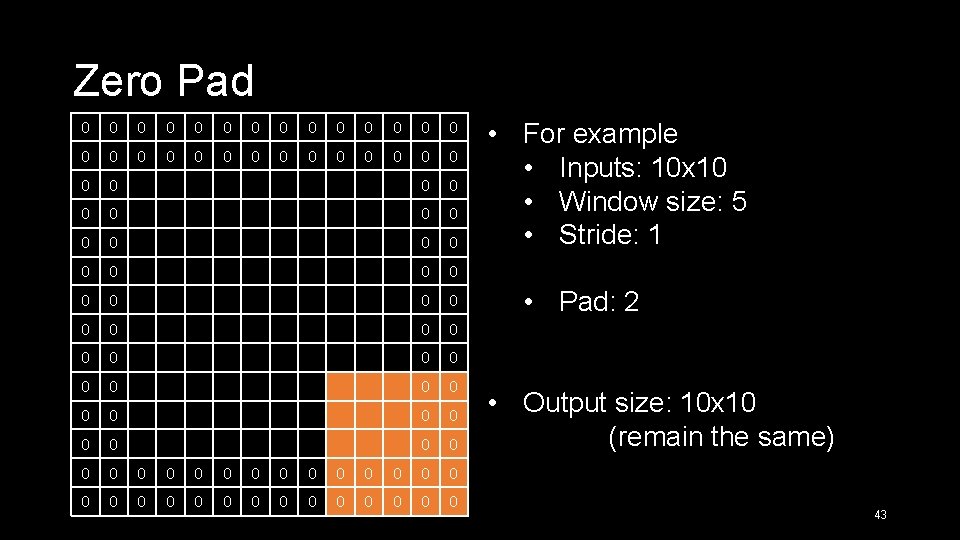
Solution to the problem of stride • Padding! • That means we add value in the border of the image. • We often add 0 in the border. 41

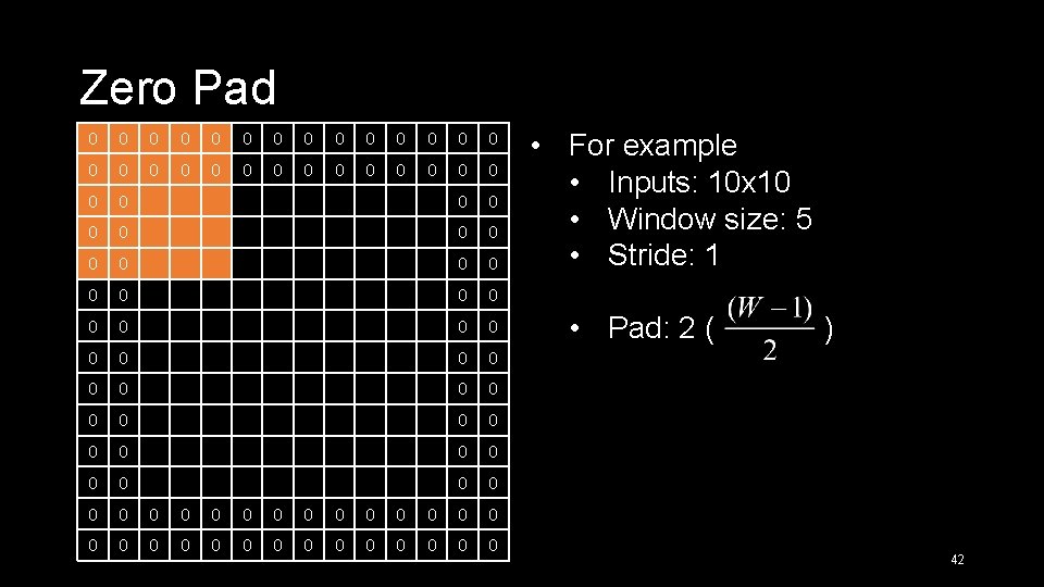
Zero Pad 0 0 0 0 0 0 0 0 0 0 0 0 0 0 0 0 0 0 0 0 0 0 0 0 • For example • Inputs: 10 x 10 • Window size: 5 • Stride: 1 • Pad: 2 ( ) 42

Zero Pad 0 0 0 0 0 0 0 0 0 0 0 0 0 0 0 0 0 0 0 0 0 0 0 0 • For example • Inputs: 10 x 10 • Window size: 5 • Stride: 1 • Pad: 2 • Output size: 10 x 10 (remain the same) 43

Padding • We can keep the output size by padding. • Besides, we can avoid the border information “washing out”. 44

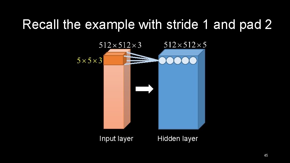
Recall the example with stride 1 and pad 2 Input layer Hidden layer 45

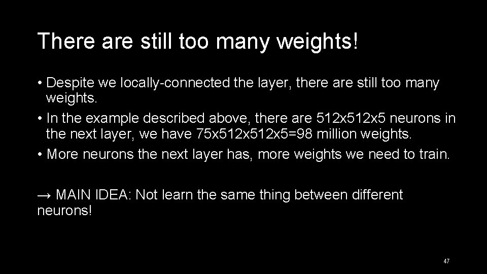
There are still too many weights! • Despite we locally-connected the layer, there are still too many weights. • In the example described above, there are 512 x 5 neurons in the next layer, we have 75 x 512 x 5=98 million weights. • More neurons the next layer has, more weights we need to train. 46

There are still too many weights! • Despite we locally-connected the layer, there are still too many weights. • In the example described above, there are 512 x 5 neurons in the next layer, we have 75 x 512 x 5=98 million weights. • More neurons the next layer has, more weights we need to train. → MAIN IDEA: Not learn the same thing between different neurons! 47

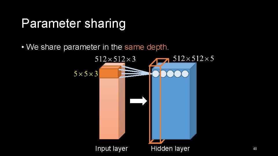
Parameter sharing • We share parameter in the same depth. Input layer Hidden layer 48

Parameter sharing • We share parameter in the same depth. • Now we only have 75 x 5=375 weights. 49

Two Main Idea in CNNs • Local connected • Parameter sharing • Cause that is like we apply convolution on the image, we call this neural network CNN. • We call these layers “convolution layers”. • What we learn can be considered as the convolution filters. 50

Other layers in the CNNs • Pool layer • Fully-connected layer 51

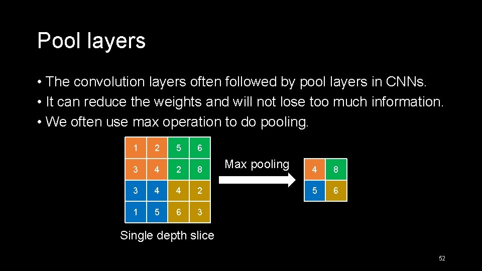
Pool layers • The convolution layers often followed by pool layers in CNNs. • It can reduce the weights and will not lose too much information. • We often use max operation to do pooling. 1 2 5 6 3 4 2 8 3 4 4 2 1 5 6 3 Max pooling 4 8 5 6 Single depth slice 52

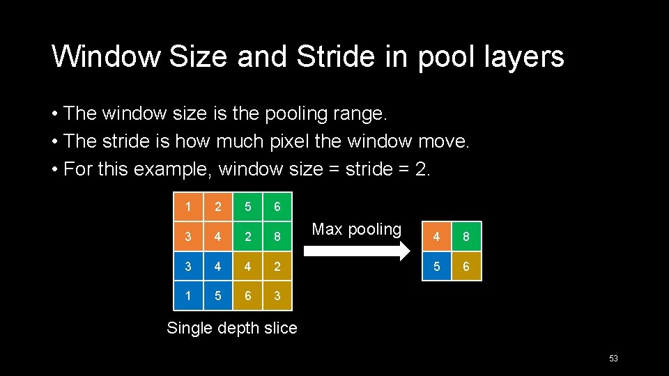
Window Size and Stride in pool layers • The window size is the pooling range. • The stride is how much pixel the window move. • For this example, window size = stride = 2. 1 2 5 6 3 4 2 8 3 4 4 2 1 5 6 3 Max pooling 4 8 5 6 Single depth slice 53

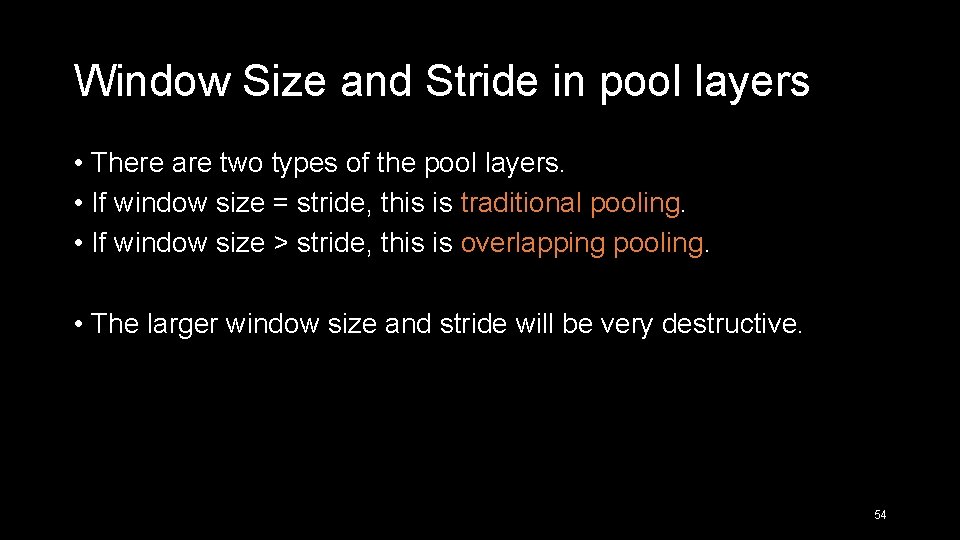
Window Size and Stride in pool layers • There are two types of the pool layers. • If window size = stride, this is traditional pooling. • If window size > stride, this is overlapping pooling. • The larger window size and stride will be very destructive. 54

Fully-connected layer • This layer is the same as the layer in the traditional NNs. • We often use this type of layers in the end of the CNNs. 55

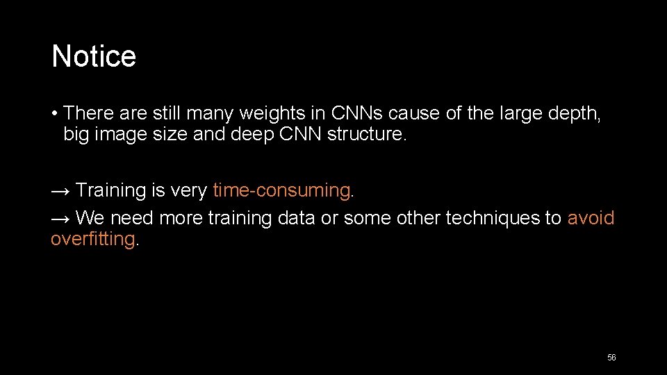
Notice • There are still many weights in CNNs cause of the large depth, big image size and deep CNN structure. → Training is very time-consuming. → We need more training data or some other techniques to avoid overfitting. 56

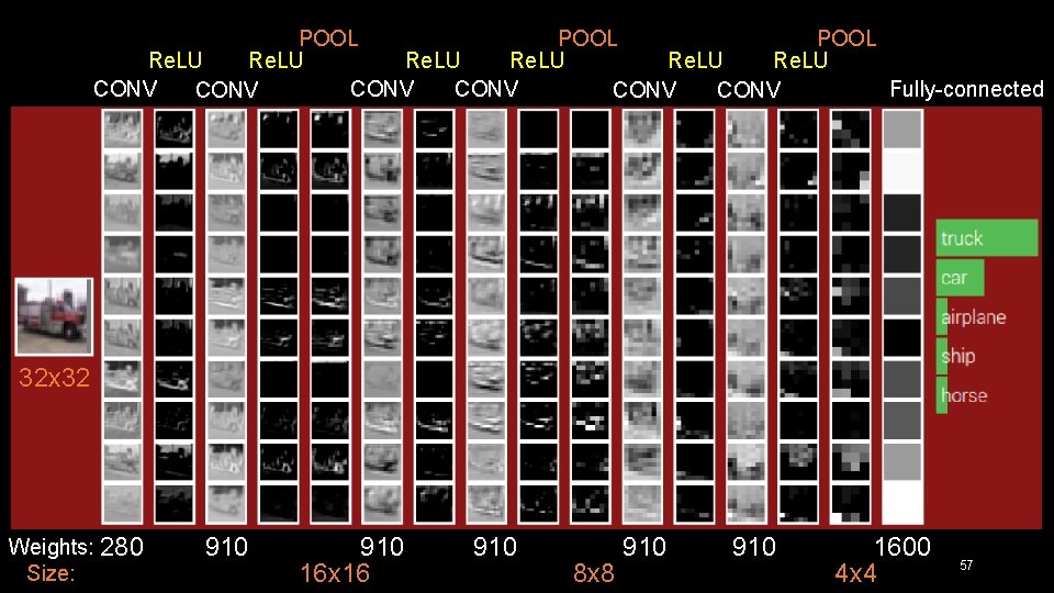
POOL Re. LU Fully-connected CONV CONV 32 x 32 Weights: 280 Size: 910 16 x 16 910 8 x 8 910 1600 4 x 4 57

Outline • Neural Networks • Convolutional Neural Networks • Some famous CNN structure • Applications • Toolkit • Conclusion • Reference 58

Le. Net-5 [8] (Le. Cun, 1998) [8] 59

Alex. Net [9] (Alex, 1998) [9] 60

VGGNet [12] 61

Outline • Neural Networks • Convolutional Neural Networks • Some famous CNN structure • Applications • Toolkit • Conclusion • Reference 62

Object classification [9] 63

Human Pose Estimation [10] 64

Super Resolution [11] 65

Outline • Neural Networks • Convolutional Neural Networks • Some famous CNN structure • Applications • Toolkit • Conclusion • Reference 66

Caffe • Developed by the University of California. • Operating system: Linux • Coding environment: Python • Can use NVIDIA CUDA GPU machine to speed up. 67

Outline • Neural Networks • Convolutional Neural Networks • Some famous CNN structure • Applications • Toolkit • Conclusion • Reference 68

Conclusion • The CNNs are based on locally-connected and parameter sharing. • Though we can get good performance by using CNNs, there are two things we need to notice, time-consuming and overfitting. • Sometimes we use pretrained models instead of training a new structure. 69

Outline • Neural Networks • Convolutional Neural Networks • Some famous CNN structure • Applications • Toolkit • Conclusion • Reference 70

Reference • Image [1] http: //4. bp. blogspot. com/-l 9 l. Ukj. LHuhg/Upp. KPZ-FCI/AAAABw. U/W 3 DGUFCm. UGY/s 1600/brain-neural-map. jpg [2] http: //wave. engr. uga. edu/images/neuron. jpg [3] http: //www. codeproject. com/KB/recipes/Neural. Network_1/NN 2. png [4] http: //wwwold. ece. utep. edu/research/webfuzzy/docs/kk-thesis/kkthesis-html/img 17. gif [5] http: //stackoverflow. com/questions/2480650/role-of-bias-in-neuralnetworks [6] http: //vision. stanford. edu/teaching/cs 231 n/slides/lecture 7. pdf [7] http: //www. cs. nott. ac. uk/~pszgxk/courses/g 5 aiai/006 neuralnetworks /images/actfn 001. jpg [13] http: //mathworld. wolfram. com/Sigmoid. Function. html 71 [14] http: //cs 231 n. github. io/assets/nn 1/relu. jpeg

Reference • Paper [8] Le. Cun, Y. , Bottou, L. , Bengio, Y. , & Haffner, P. (1998). Gradientbased learning applied to document recognition. Proceedings of the IEEE, 86(11), 2278 -2324. [9] Krizhevsky, Alex, Ilya Sutskever, and Geoffrey E. Hinton. "Imagenet classification with deep convolutional neural networks. " Advances in neural information processing systems. 2012. [10] Toshev, Alexander, and Christian Szegedy. "Deeppose: Human pose estimation via deep neural networks. " Computer Vision and Pattern Recognition (CVPR), 2014 IEEE Conference on. IEEE, 2014. [11] Dong, C. , Loy, C. C. , He, K. , & Tang, X. (2014). Image Super. Resolution Using Deep Convolutional Networks. ar. Xiv preprint ar. Xiv: 1501. 00092. [12] Simonyan, Karen, and Andrew Zisserman. "Very deep convolutional networks for large-scale image recognition. " ar. Xiv preprint ar. Xiv: 1409. 1556 (2014). 72