Convergence and Divergence in Growth Regressions Michele Battisti

Convergence and Divergence in Growth Regressions Michele Battisti University of Palermo Gianfranco di Vaio Cassa Depositi e Prestiti Joseph Zeira Hebrew University of Jerusalem and LUISS Jerusalem, June 19, 2014

Introduction • This paper extends the main model of growth regressions (Barro 1991 and later), in order to overcome a number of critiques on this literature. • One main result of growth regressions is that the cross-country distribution of output converges to a limit distribution. But direct studies of this distribution (Bernard and Durlauf 1995 and more) found that it diverges over time. • The choice of control variables for estimation of convergence is arbitrary and their total number already exceeds 150. • Measures of the rate of convergence differ across studies.

Introduction: Main Results • Our extended model of growth regression enables us to reconcile the conflicting results of convergence and divergence. • We succeed in estimating the dynamic parameters of the model without use of any control variables. • We provide an explanation to different estimates of the rate of convergence. • We can isolate the long-run effect of explanatory variables, which cannot be done in standard growth regressions.

Introduction: Our Extension • The standard growth regression model assumes that the ratio between output per worker of a country and its productivity (TFP) converges at an annual rate b to a constant number. • We add an assumption on how productivity evolves over time: it converges to a long-run path at a rate c. • This long-run path follows the global technology (or productivity) frontier. But it may follow it only partially. • We assume that each country has a parameter d that measures by how much it follows the global frontier in the long-run. If d = 1 it follows fully, and if d < 1, it follows partially.

Introduction: Justification and Implications • Our approach can be described as growth in small open economies. Most countries do not invent new technologies, but use the innovations created elsewhere. They can either adopt an innovation, or not. Hence, d might be smaller than 1. • The model implies that growth is characterized by 3 parameters: b measures convergence of output, c measures convergence of productivity, and d measures divergence from the frontier. • We estimate the 3 parameters and find that d is below 1 for many countries (the global average is 0. 7).

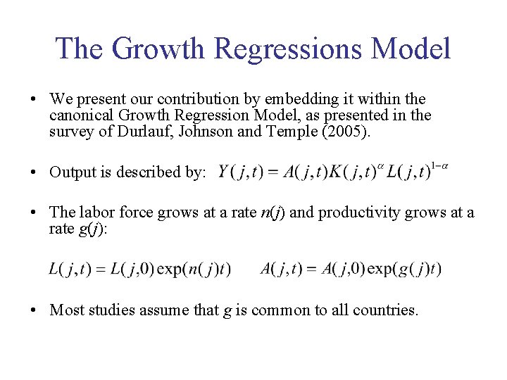
The Growth Regressions Model • We present our contribution by embedding it within the canonical Growth Regression Model, as presented in the survey of Durlauf, Johnson and Temple (2005). • Output is described by: • The labor force grows at a rate n(j) and productivity grows at a rate g(j): • Most studies assume that g is common to all countries.

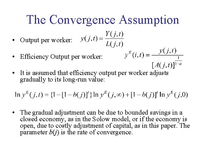
The Convergence Assumption • Output per worker: • Efficiency Output per worker: • It is assumed that efficiency output per worker adjusts gradually to its long-run value: • The gradual adjustment can be due to bounded savings in a closed economy, as in the Solow model, or if the economy is open, due to costly adjustment of capital, as in this paper. The parameter b(j) is the rate of convergence.

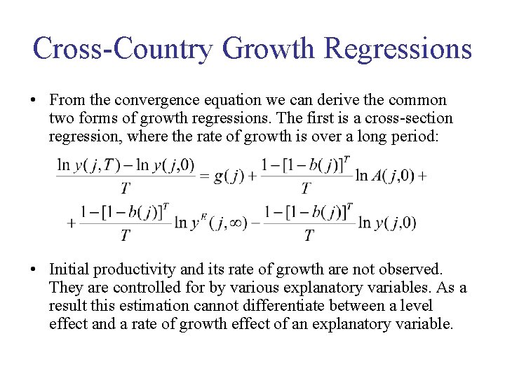
Cross-Country Growth Regressions • From the convergence equation we can derive the common two forms of growth regressions. The first is a cross-section regression, where the rate of growth is over a long period: • Initial productivity and its rate of growth are not observed. They are controlled for by various explanatory variables. As a result this estimation cannot differentiate between a level effect and a rate of growth effect of an explanatory variable.

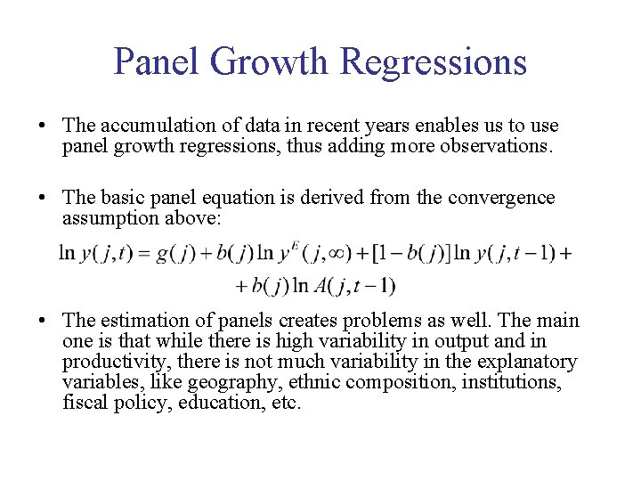
Panel Growth Regressions • The accumulation of data in recent years enables us to use panel growth regressions, thus adding more observations. • The basic panel equation is derived from the convergence assumption above: • The estimation of panels creates problems as well. The main one is that while there is high variability in output and in productivity, there is not much variability in the explanatory variables, like geography, ethnic composition, institutions, fiscal policy, education, etc.

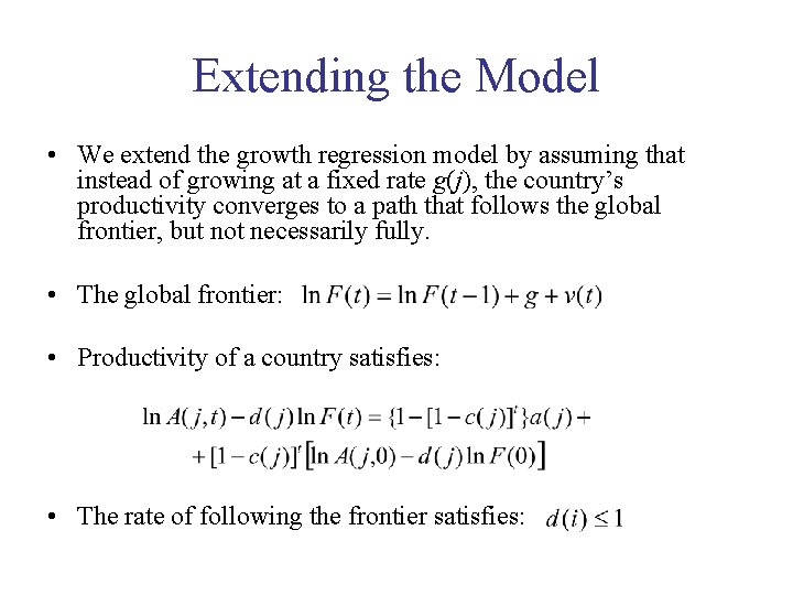
Extending the Model • We extend the growth regression model by assuming that instead of growing at a fixed rate g(j), the country’s productivity converges to a path that follows the global frontier, but not necessarily fully. • The global frontier: • Productivity of a country satisfies: • The rate of following the frontier satisfies:

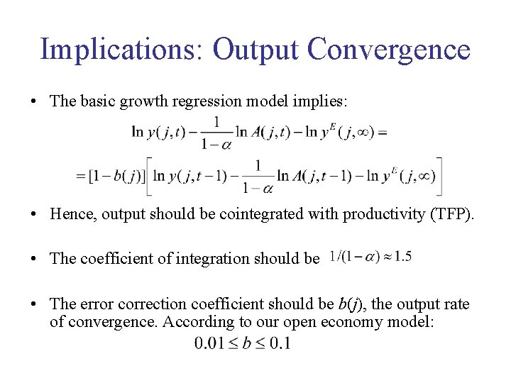
Implications: Output Convergence • The basic growth regression model implies: • Hence, output should be cointegrated with productivity (TFP). • The coefficient of integration should be • The error correction coefficient should be b(j), the output rate of convergence. According to our open economy model:

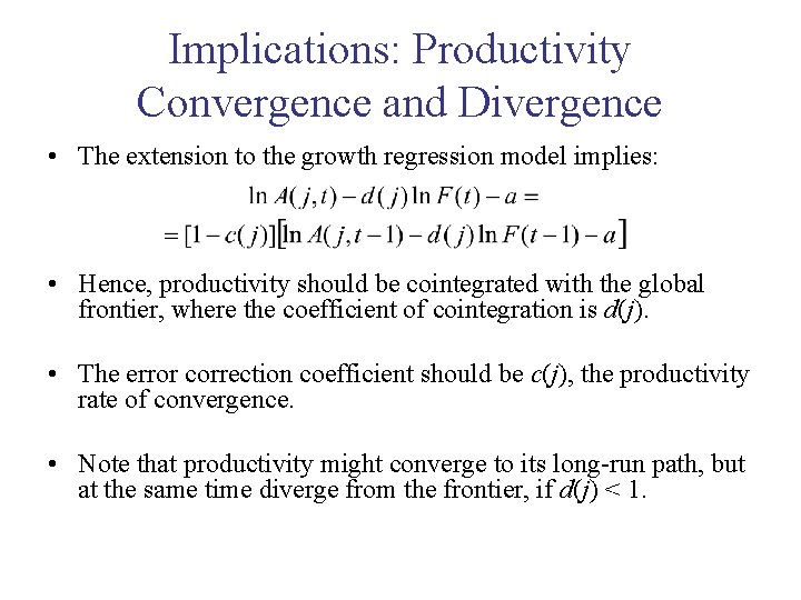
Implications: Productivity Convergence and Divergence • The extension to the growth regression model implies: • Hence, productivity should be cointegrated with the global frontier, where the coefficient of cointegration is d(j). • The error correction coefficient should be c(j), the productivity rate of convergence. • Note that productivity might converge to its long-run path, but at the same time diverge from the frontier, if d(j) < 1.

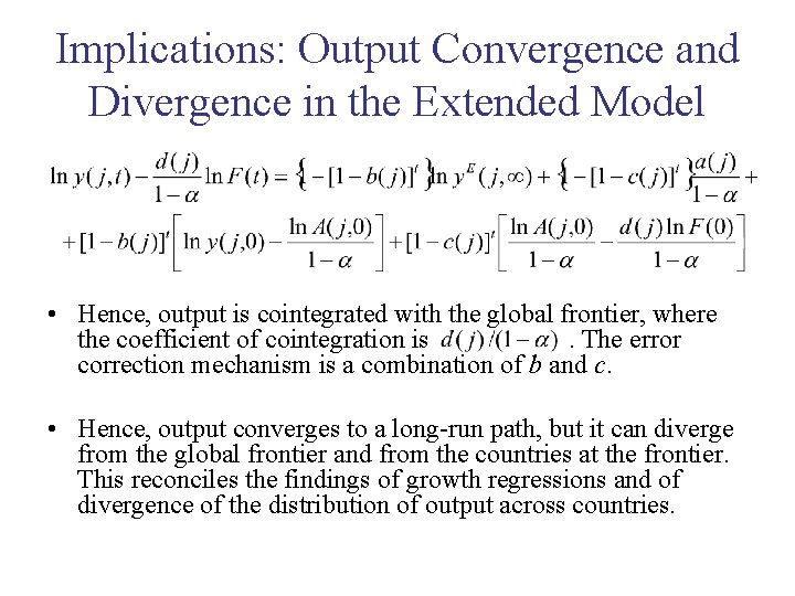
Implications: Output Convergence and Divergence in the Extended Model • Hence, output is cointegrated with the global frontier, where the coefficient of cointegration is. The error correction mechanism is a combination of b and c. • Hence, output converges to a long-run path, but it can diverge from the global frontier and from the countries at the frontier. This reconciles the findings of growth regressions and of divergence of the distribution of output across countries.

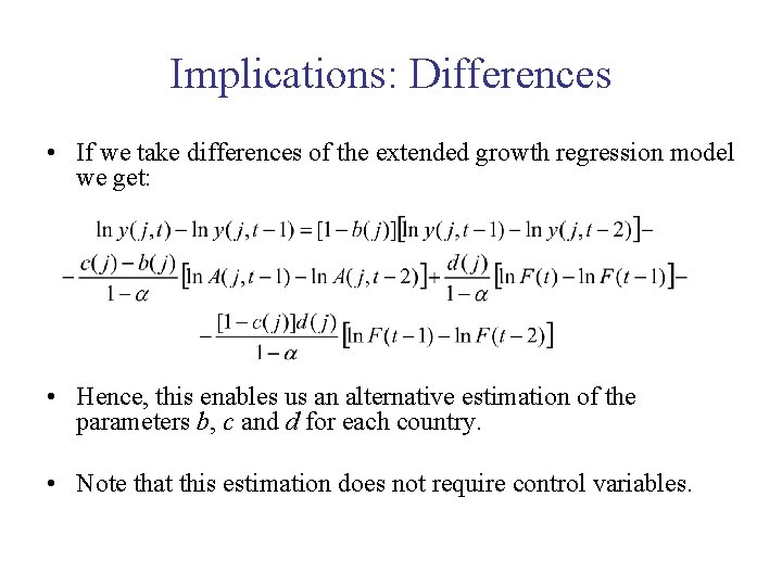
Implications: Differences • If we take differences of the extended growth regression model we get: • Hence, this enables us an alternative estimation of the parameters b, c and d for each country. • Note that this estimation does not require control variables.

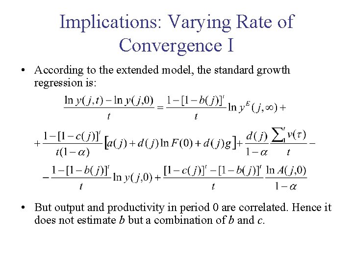
Implications: Varying Rate of Convergence I • According to the extended model, the standard growth regression is: • But output and productivity in period 0 are correlated. Hence it does not estimate b but a combination of b and c.

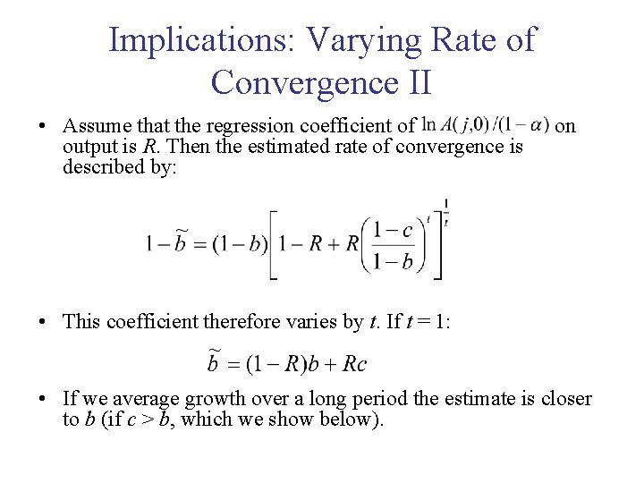
Implications: Varying Rate of Convergence II • Assume that the regression coefficient of output is R. Then the estimated rate of convergence is described by: on • This coefficient therefore varies by t. If t = 1: • If we average growth over a long period the estimate is closer to b (if c > b, which we show below).

Data • We use data on output per capita, which is PPP adjusted, from the Groningen Growth and Development Centre (2013). • Specifically, real GDP per capita, in PPP adjusted Geary. Khamis 1990 US$, for 139 countries over the years 1950 -2008. We remove a few outliers (like oil producing countries) and are left with 124 countries. • For a set of 30 countries the data are from 1870 to 2010. • For the global frontier we use as a proxy the US output per capita. The US has a stable growth rate over the period and is the leading among large countries.

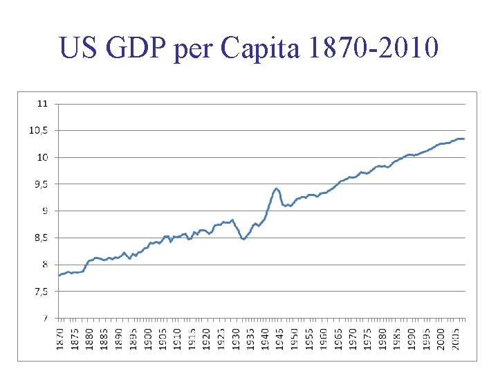
US GDP per Capita 1870 -2010

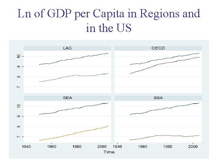
Ln of GDP per Capita in Regions and in the US

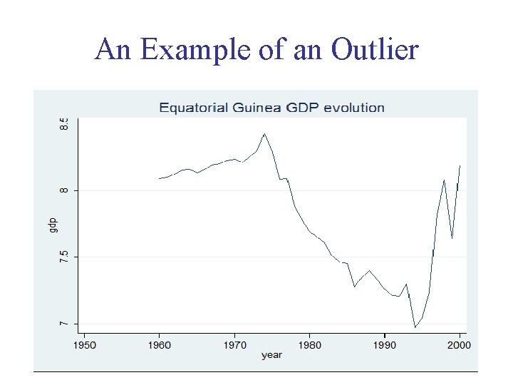
An Example of an Outlier

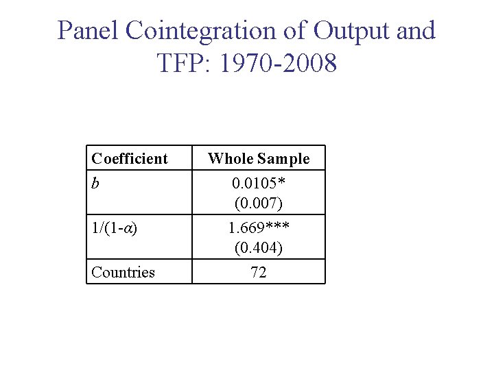
Panel Cointegration of Output and TFP: 1970 -2008 Coefficient b 1/(1 -α) Countries Whole Sample 0. 0105* (0. 007) 1. 669*** (0. 404) 72

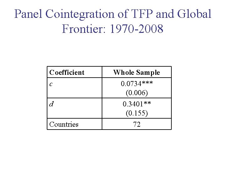
Panel Cointegration of TFP and Global Frontier: 1970 -2008 Coefficient c d Countries Whole Sample 0. 0734*** (0. 006) 0. 3401** (0. 155) 72

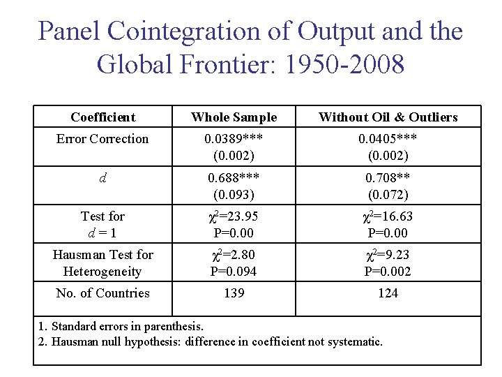
Panel Cointegration of Output and the Global Frontier: 1950 -2008 Coefficient Whole Sample Without Oil & Outliers Error Correction 0. 0389*** (0. 002) 0. 0405*** (0. 002) d 0. 688*** (0. 093) 0. 708** (0. 072) Test for d=1 χ2=23. 95 P=0. 00 χ2=16. 63 P=0. 00 Hausman Test for Heterogeneity χ2=2. 80 P=0. 094 χ2=9. 23 P=0. 002 No. of Countries 139 124 1. Standard errors in parenthesis. 2. Hausman null hypothesis: difference in coefficient not systematic.

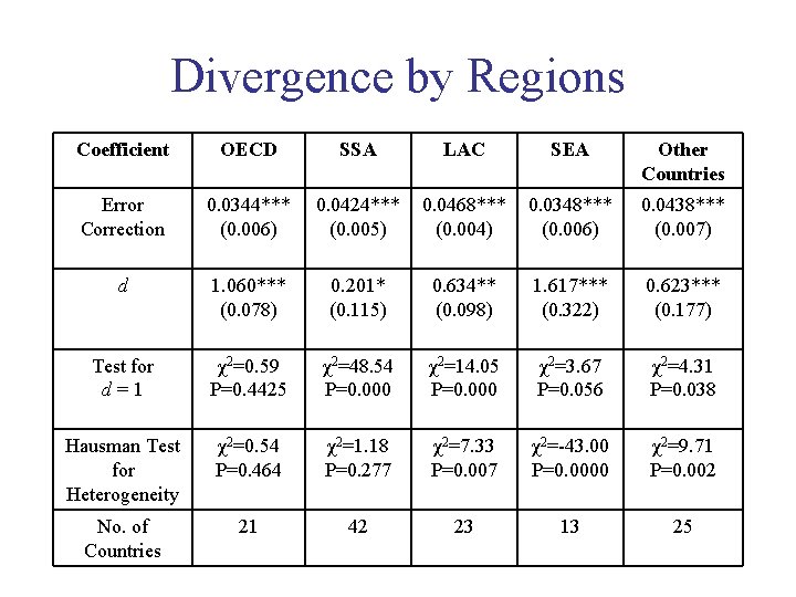
Divergence by Regions Coefficient OECD SSA LAC SEA Other Countries Error Correction 0. 0344*** (0. 006) 0. 0424*** (0. 005) 0. 0468*** (0. 004) 0. 0348*** (0. 006) 0. 0438*** (0. 007) d 1. 060*** (0. 078) 0. 201* (0. 115) 0. 634** (0. 098) 1. 617*** (0. 322) 0. 623*** (0. 177) Test for d=1 χ2=0. 59 P=0. 4425 χ2=48. 54 P=0. 000 χ2=14. 05 P=0. 000 χ2=3. 67 P=0. 056 χ2=4. 31 P=0. 038 Hausman Test for Heterogeneity χ2=0. 54 P=0. 464 χ2=1. 18 P=0. 277 χ2=7. 33 P=0. 007 χ2=-43. 00 P=0. 0000 χ2=9. 71 P=0. 002 No. of Countries 21 42 23 13 25

Convergence and Divergence • In all regressions countries follow what is called βconvergence, or conditional convergence. • But here this is interpreted as convergence to own long-run growth path. • But the long-run path may converge to the frontier or diverge from it, depending on whether d = 1 or smaller than 1. • We show that for most countries d < 1, so that most countries diverge from the frontier. This fits the many findings on divergence.

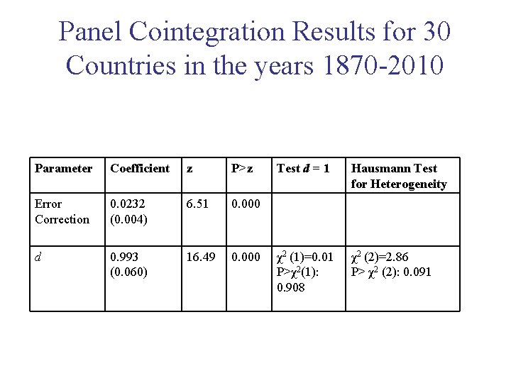
Panel Cointegration Results for 30 Countries in the years 1870 -2010 Parameter Coefficient z P>z Error Correction 0. 0232 (0. 004) 6. 51 0. 000 d 0. 993 (0. 060) 16. 49 0. 000 Test d = 1 Hausmann Test for Heterogeneity χ2 (1)=0. 01 P>χ2(1): 0. 908 χ2 (2)=2. 86 P> χ2 (2): 0. 091

Effect of Explanatory Variables on d • Next we estimate the effect of various explanatory variables on the estimated d. • Previous growth regressions could estimate whether an explanatory variable affects output. • The effects of these same explanatory variables on d can identify their long-run effect. • We compare this estimation with a standard growth regression to check whether these long-run effect actually differ from the overall effect.

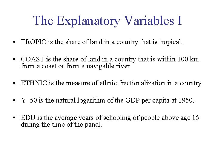
The Explanatory Variables I • TROPIC is the share of land in a country that is tropical. • COAST is the share of land in a country that is within 100 km from a coast or from a navigable river. • ETHNIC is the measure of ethnic fractionalization in a country. • Y_50 is the natural logarithm of the GDP per capita at 1950. • EDU is the average years of schooling of people above age 15 during the time of the panel.

The Explanatory Variables II • OPEN measures openness by trade policy over the years 19651990. A country is closed (i) if average tariff rate exceeded 40%; (ii) if non-tariff barriers covered more than 40% of imports; (iii) if it had a socialist economic system; (iv) if it had a state monopoly of major exports; or (v) if black-market premium exceeded 20% during the 1970 s or the 1980 s. • ICRG is average measure of quality of institutions during 1982 -1997 (International Country Risk Guide). • G/Y is the share of public expenditures in GDP, averaged over the years 1950 -1960.

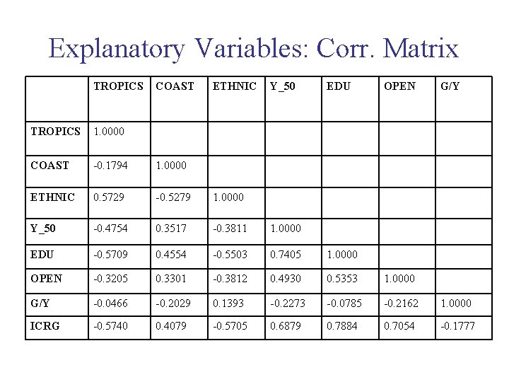
Explanatory Variables: Corr. Matrix TROPICS COAST ETHNIC Y_50 EDU OPEN G/Y TROPICS 1. 0000 COAST -0. 1794 1. 0000 ETHNIC 0. 5729 -0. 5279 1. 0000 Y_50 -0. 4754 0. 3517 -0. 3811 1. 0000 EDU -0. 5709 0. 4554 -0. 5503 0. 7405 1. 0000 OPEN -0. 3205 0. 3301 -0. 3812 0. 4930 0. 5353 1. 0000 G/Y -0. 0466 -0. 2029 0. 1393 -0. 2273 -0. 0785 -0. 2162 1. 0000 ICRG -0. 5740 0. 4079 -0. 5705 0. 6879 0. 7884 0. 7054 -0. 1777

Taking Out SEA and OECD • In the following regressions we estimate the effects of these explanatory variables (except for ICRG, for insignificance) for all countries and then without South East Asia and even without the OECD countries. • Some of the South East Asian countries are in the midst of a period of catching up with the frontier so their rate of growth is very high and they appear to have d that is much higher than 1. We know that this catching up will stop some time, but the data do not know. • The OECD countries have d = 1, which is the maximum d. Hence they are at a corner solution, so that d is less sensitive to the various explanatory variables.

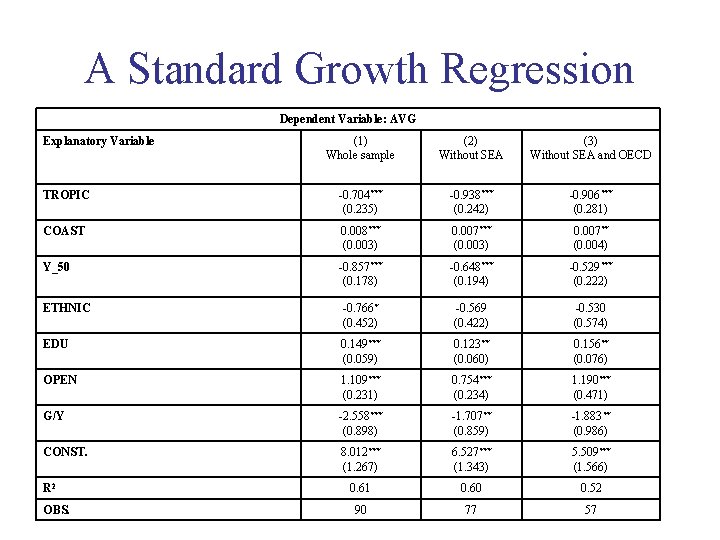
A Standard Growth Regression Dependent Variable: AVG Explanatory Variable (1) Whole sample (2) Without SEA (3) Without SEA and OECD TROPIC -0. 704*** (0. 235) -0. 938*** (0. 242) -0. 906*** (0. 281) COAST 0. 008*** (0. 003) 0. 007** (0. 004) Y_50 -0. 857*** (0. 178) -0. 648*** (0. 194) -0. 529*** (0. 222) ETHNIC -0. 766* (0. 452) -0. 569 (0. 422) -0. 530 (0. 574) EDU 0. 149*** (0. 059) 0. 123** (0. 060) 0. 156** (0. 076) OPEN 1. 109*** (0. 231) 0. 754*** (0. 234) 1. 190*** (0. 471) G/Y -2. 558*** (0. 898) -1. 707** (0. 859) -1. 883** (0. 986) CONST. 8. 012*** (1. 267) 6. 527*** (1. 343) 5. 509*** (1. 566) 0. 61 0. 60 0. 52 90 77 57 R 2 OBS.

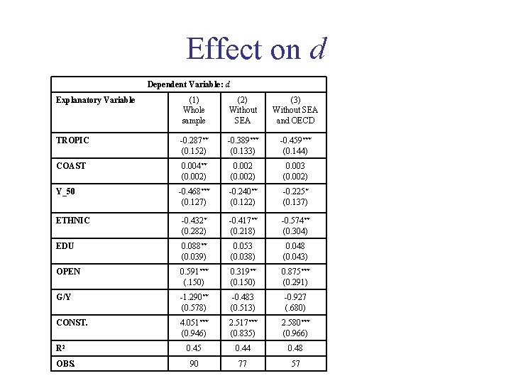
Effect on d Dependent Variable: d Explanatory Variable (1) Whole sample (2) Without SEA (3) Without SEA and OECD TROPIC -0. 287** (0. 152) -0. 389*** (0. 133) -0. 459*** (0. 144) COAST 0. 004** (0. 002) 0. 002 (0. 002) 0. 003 (0. 002) -0. 468*** (0. 127) -0. 240** (0. 122) -0. 225* (0. 137) ETHNIC -0. 432* (0. 282) -0. 417** (0. 218) -0. 574** (0. 304) EDU 0. 088** (0. 039) 0. 053 (0. 038) 0. 048 (0. 043) OPEN 0. 591*** (. 150) 0. 319** (0. 150) 0. 875*** (0. 291) G/Y -1. 290** (0. 578) -0. 483 (0. 513) -0. 927 (. 680) CONST. 4. 051*** (0. 946) 2. 517*** (0. 835) 2. 580*** (0. 966) 0. 45 0. 44 0. 48 90 77 57 Y_50 R 2 OBS.

Results • The effects of explanatory variables in the standard crosscountry growth regression are very different from the effects on d. • Education has a positive and significant effect on growth, but not on d. • The size of the public sector has a significant negative effect on output in growth regression, but its effect on d is insignificant. • The effect of ethnic fractionalization on output is insignificant, but its effect on long-run growth is negative and significant.

Conclusions • It is still a bit too early to throw growth regressions into the dump. • Including the global frontier and productivity can enrich the estimation of convergence and divergence of countries. • We reconcile the results of growth regressions with alternative measures of convergence and divergence. We also estimate convergence without control variables. We also improve the estimation of the rate of convergence. • This approach also enables us to better evaluate various explanations to growth, by isolating the long-run effect.

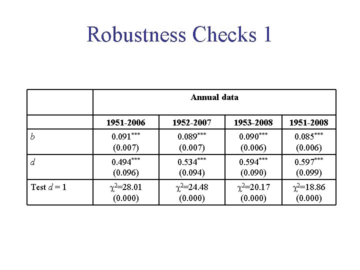
Robustness Checks 1 Annual data 1951 -2006 1952 -2007 1953 -2008 1951 -2008 b 0. 091*** (0. 007) 0. 089*** (0. 007) 0. 090*** (0. 006) 0. 085*** (0. 006) d 0. 494*** (0. 096) 0. 534*** (0. 094) 0. 594*** (0. 090) 0. 597*** (0. 099) Test d = 1 2=28. 01 (0. 000) 2=24. 48 (0. 000) 2=20. 17 (0. 000) 2=18. 86 (0. 000)

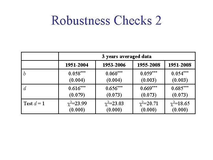
Robustness Checks 2 3 years averaged data 1951 -2004 1953 -2006 1955 -2008 1951 -2008 b 0. 058*** (0. 004) 0. 060*** (0. 004) 0. 059*** (0. 003) 0. 054*** (0. 003) d 0. 616*** (0. 079) 0. 656*** (0. 073) 0. 669*** (0. 073) 0. 685*** (0. 073) Test d = 1 2=23. 99 (0. 000) 2=23. 03 (0. 000) 2=20. 71 (0. 000) 2=18. 65 (0. 000)

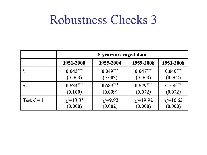
Robustness Checks 3 5 years averaged data 1951 -2000 1955 -2004 1959 -2008 1951 -2008 b 0. 045*** (0. 003) 0. 049*** (0. 003) 0. 047*** (0. 003) 0. 040*** (0. 002) d 0. 634*** (0. 100) 0. 689*** (0. 099) 0. 679*** (0. 072) 0. 708*** (0. 072) Test d = 1 2=13. 35 (0. 000) 2=9. 82 (0. 002) 2=19. 92 (0. 000) 2=16. 63 (0. 000)

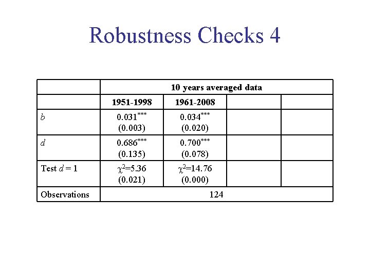
Robustness Checks 4 10 years averaged data 1951 -1998 1961 -2008 b 0. 031*** (0. 003) 0. 034*** (0. 020) d 0. 686*** (0. 135) 0. 700*** (0. 078) Test d = 1 2=5. 36 (0. 021) 2=14. 76 (0. 000) Observations 124

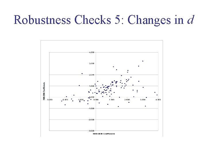
Robustness Checks 5: Changes in d

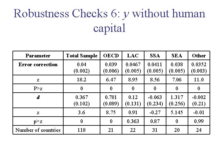
Robustness Checks 6: y without human capital Parameter Total Sample OECD LAC SSA SEA Other Error correction 0. 04 (0. 002) 0. 039 (0. 006) 0. 0467 (0. 005) 0. 0411 (0. 005) 0. 038 (0. 005) 0. 0352 (0. 003) z 18. 2 6. 47 8. 95 8. 56 7. 06 11. 0 P>z 0 0 0 d 0. 367 (0. 102) 0. 781 (0. 089) 0. 12 (0. 131) -0. 063 (0. 234) 1. 317 (0. 256) -0. 002 (0. 21) z 3. 6 8. 75 0. 91 -0. 27 5. 145 -0. 01 p>z 0 0 0. 363 0. 87 0 0. 99 Number of countries 118 21 22 31 20 24