Controlling Animation BoundaryValue Problems Shooting Methods Constrained Optimization

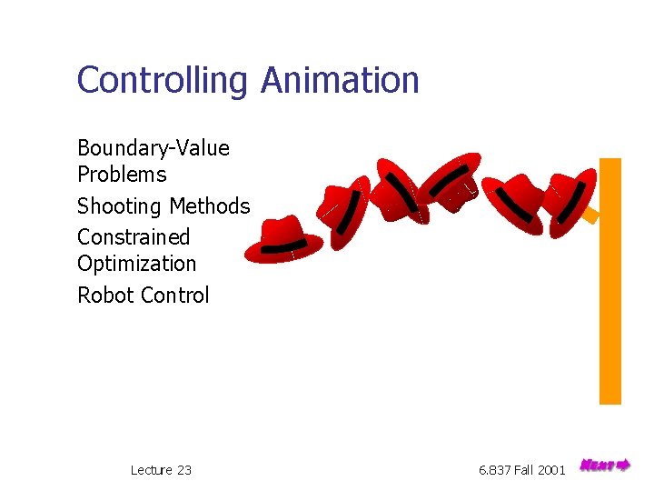
Controlling Animation Boundary-Value Problems Shooting Methods Constrained Optimization Robot Control Lecture 23 6. 837 Fall 2001

Computer Animation Story (concept, storyboard) Production (modeling, motion, lighting) Lecture 23 Slide 2 2

Motion Keyframing n n Interpolates motion from “key” positions Perfect control Can be tedious No realism Lecture 23 Slide 3 3

Motion Simulation n n Solves equations of motion to compute motion Realistic motion Automatic generation Difficult to control Lecture 23 Slide 4 4

Controlling Simulation What initial velocity will cause the hat to land on the coatrack? Lecture 23 Slide 5 5

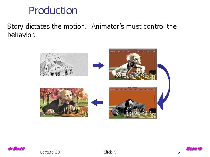
Production Story dictates the motion. Animator’s must control the behavior. Lecture 23 Slide 6 6

Simulation Function S(t, u) initial velocity simulator nonlinear not continuous Lecture 23 Slide 7 7

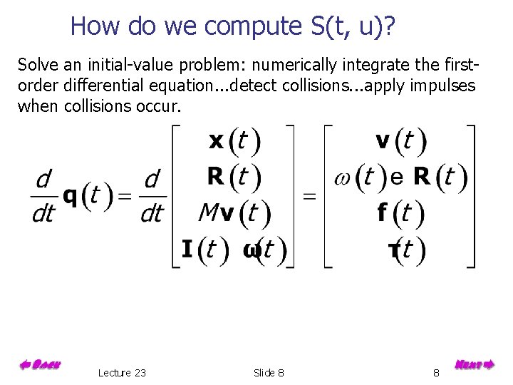
How do we compute S(t, u)? Solve an initial-value problem: numerically integrate the firstorder differential equation. . . detect collisions. . . apply impulses when collisions occur. Lecture 23 Slide 8 8

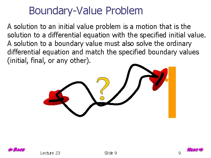
Boundary-Value Problem A solution to an initial value problem is a motion that is the solution to a differential equation with the specified initial value. A solution to a boundary value must also solve the ordinary differential equation and match the specified boundary values (initial, final, or any other). Lecture 23 Slide 9 9

Boundary-Value Problem What initial velocity will cause the hat to land on the coatrack? Lecture 23 Slide 10 10

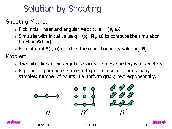
Solution by Shooting Method n n n Pick initial linear and angular velocity u = (v, ω) Simulate with initial value q 0=(x 0, R 0, u) to compute the simulation function S(t, u) Repeat until S(t, u) matches the other boundary value x 1, R 1 Problem n n The initial linear and angular velocity are described by 6 parameters. Exploring a parameter space of high-dimension requires many samples: number of points in a uniform grid grows exponentially. Lecture 23 Slide 11 11

Shooting Method We can combat the high dimensional parameter spaces with clever sampling techniques or derivative-based methods. Sampling techniques n n Importance Sampling Markov Chain Monte Carlo Derivative-based Methods n n n Gradient descent Newton’s root finding method Human assistance (interaction) Lecture 23 Slide 12 12

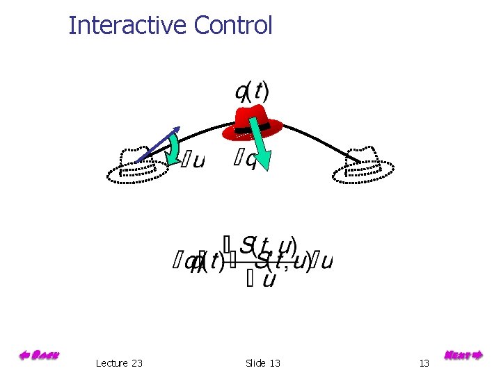
Interactive Control Lecture 23 Slide 13 13

Interactive Control Lecture 23 Slide 14 14

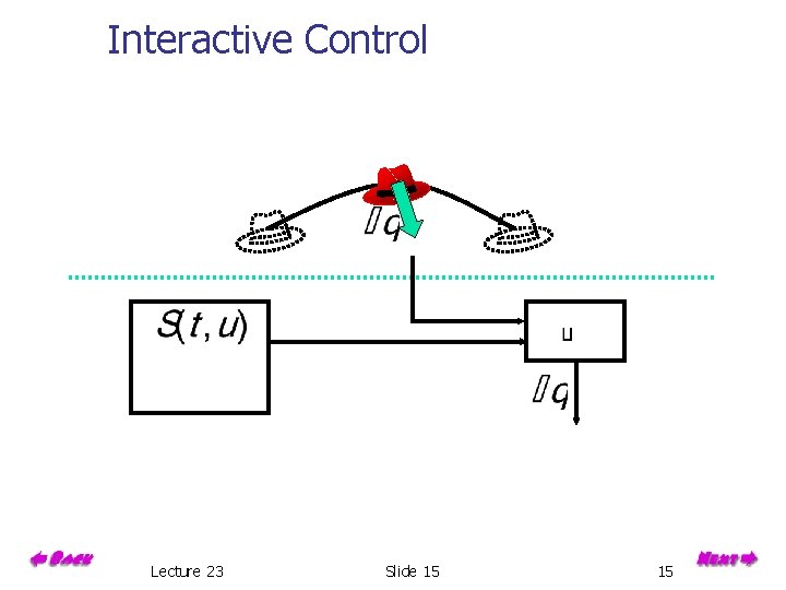
Interactive Control Lecture 23 Slide 15 15

Interactive Control update Lecture 23 Slide 16 16

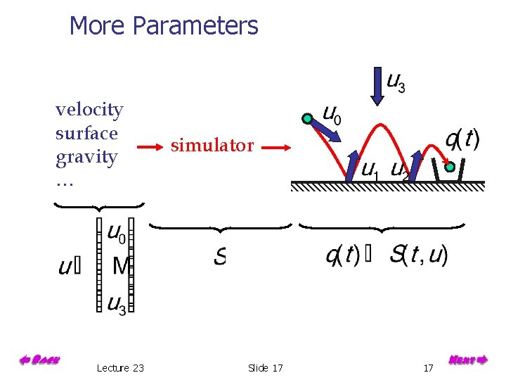
More Parameters velocity surface gravity … Lecture 23 simulator Slide 17 17

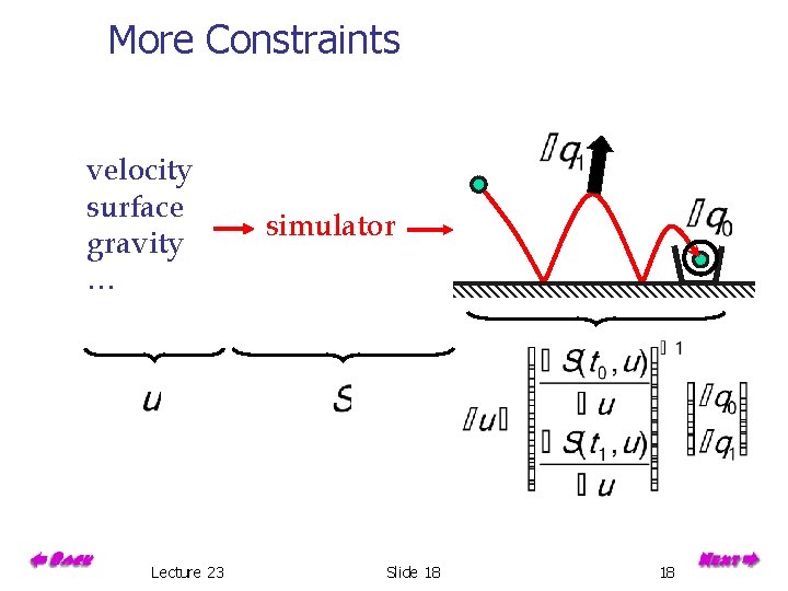
More Constraints velocity surface gravity … Lecture 23 simulator Slide 18 18

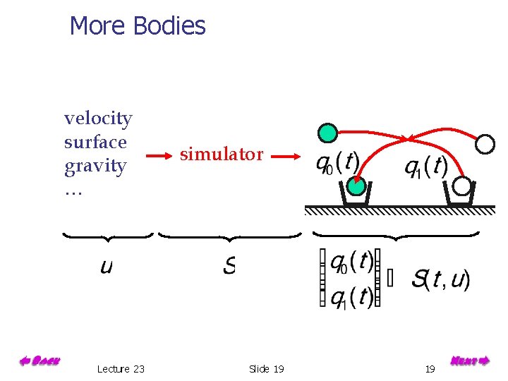
More Bodies velocity surface gravity … Lecture 23 simulator Slide 19 19

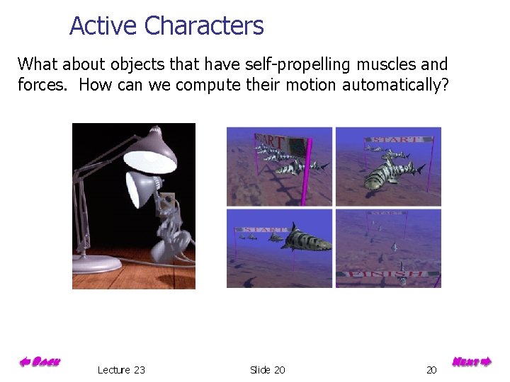
Active Characters What about objects that have self-propelling muscles and forces. How can we compute their motion automatically? Lecture 23 Slide 20 20

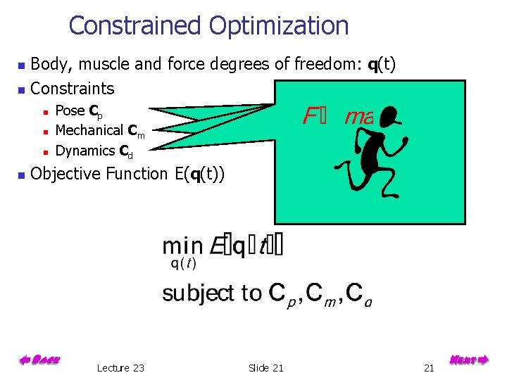
Constrained Optimization Body, muscle and force degrees of freedom: q(t) n Constraints n n n Pose Cp Mechanical Cm Dynamics Cd Objective Function E(q(t)) Lecture 23 Slide 21 21

Controller Approach Roboticists address almost identical problems in robot design. How should we control a robot to make it walk or run? Similar techniques have been applied for problems in computer animation. n n Biomechanics data and observations Feedback controllers n n designed by hand simulated annealing generate-and-test strategy parameter estimation and parallel optimization techniques Lecture 23 Slide 22 22

Next Time Research in the MIT Computer Graphics Group Lecture 23 Slide 23 23