Control Systems Lect 3 Modeling in The Time

Control Systems Lect. 3 Modeling in The Time Domain Basil Hamed

Chapter Learning Outcomes After completing this chapter, the student will be able to: • Find a mathematical model, called a state-space representation, for a linear, time invariant system (Sections 3. 1 -3. 3) • Model electrical and mechanical systems in state space (Section 3. 4) • Convert a transfer function to state space (Section 3. 5) • Convert a state-space representation to a transfer function (Section 3. 6) • Linearize a state-space representation (Section 3. 7) Basil Hamed 2

Modeling Derive mathematical models for • Electrical systems • Mechanical systems • Electromechanical system Basil Hamed Electrical Systems: • Kirchhoff’s voltage & current laws Mechanical systems: • Newton’s laws 3

3. 1 Introduction • Two approaches are available for the analysis and design of feedback control systems. The first, which we began to study in Chapter 2, is known as the classical, or frequency-domain, technique. • The 1 st approach is based on converting a system's differential equation to a transfer function, thus generating a mathematical model of the system that algebraically relates a representation of the output to a representation of the input. • The primary disadvantage of the classical approach is its limited applicability: It can be applied only to linear, timeinvariant systems or systems that can be approximated as such. Basil Hamed 4

3. 1 Introduction • The 2 nd approach is state-space approach (also referred to as the modern, or time-domain, approach) is a unified method for modeling, analyzing, and designing a wide range of systems. • For example, the state-space approach can be used to represent nonlinear systems, Time-varying systems, Multipleinput, multiple-output systems. • The time-domain approach can also be used for the same class of systems modeled by the classical approach. Basil Hamed 5

3. 2 Some Observations • We proceed now to establish the state-space approach as an alternate method for representing physical systems. • In general, an nth-order differential equation can be decomposed into n first-order differential equations. • Because, in principle, first-order differential equations are simpler to solve than higher-order ones, first-order differential equations are used in the analytical studies of control systems. Basil Hamed 6

3. 2 Some Observations Definition of State Variables The state of a system refers to the past, present, and future conditions of the system. From a mathematical perspective, it is convenient to define a set of state variables and state equations to model dynamic systems. As it turns out, the variables x 1(t), x 2(t), . . . , x„(t) are the state variables of the nth-order system Basil Hamed 7

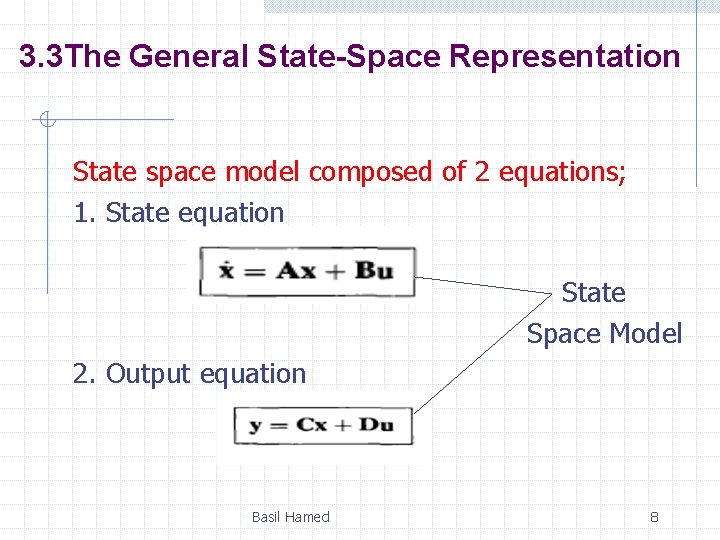
3. 3 The General State-Space Representation State space model composed of 2 equations; 1. State equation State Space Model 2. Output equation Basil Hamed 8

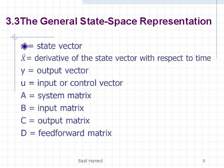
3. 3 The General State-Space Representation Basil Hamed 9

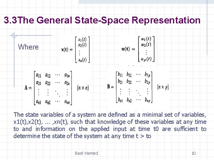
3. 3 The General State-Space Representation Where The state variables of a system are defined as a minimal set of variables, x 1(t), x 2(t), . . . , xn(t), such that knowledge of these variables at any time to and information on the applied input at time t 0 are sufficient to determine the state of the system at any time t > to Basil Hamed 10

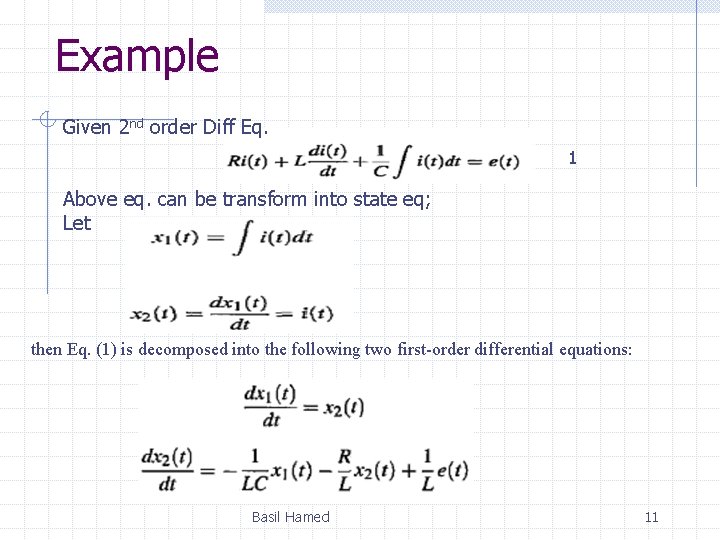
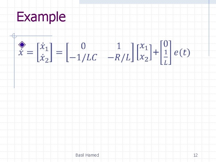
Example Given 2 nd order Diff Eq. 1 Above eq. can be transform into state eq; Let then Eq. (1) is decomposed into the following two first-order differential equations: Basil Hamed 11

Example Basil Hamed 12

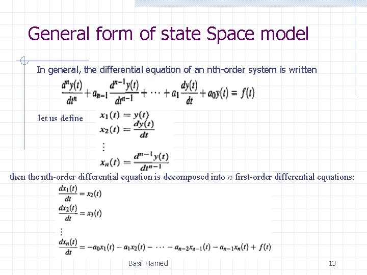
General form of state Space model In general, the differential equation of an nth-order system is written let us define then the nth-order differential equation is decomposed into n first-order differential equations: Basil Hamed 13

3. 4 Applying the State-Space Representation In this section, we apply the state-space formulation to the representation of more complicated physical systems. The first step in representing a system is to select the state vector, which must be chosen according to the following considerations: 1. A minimum number of state variables must be selected as components of the state vector. This minimum number of state variables is sufficient to describe completely the state of the system. 2. The components of the state vector (that is, this minimum number of state variables) must be linearly independent. Basil Hamed 14

Linearly Independent State Variables The components of the state vector must be linearly independent. For example, following the definition of linear independence, if x 1, x 2, and x 3 are chosen as state variables, but x 3 = 5 x 1 + 4 x 2, then x 3 is not linearly independent of x 1 and x 2, since knowledge of the values of x 1 and x 2 will yield the value of x 3. Basil Hamed 15

Minimum Number of State Variables • Typically, the minimum number required equals the order of the differential equation describing the system. For example, if a third-order differential equation describes the system, then three simultaneous, first-order differential equations are required along with three state variables. • From the perspective of the transfer function, the order of the differential equation is the order of the denominator of the transfer function after canceling common factors in the numerator and denominator. Basil Hamed 16

Minimum Number of State Variables • In most cases, another way to determine the number of state variables is to count the number of independent energystorage elements in the system. • The number of these energy-storage elements equals the order of the differential equation and the number of state variables. Basil Hamed 17

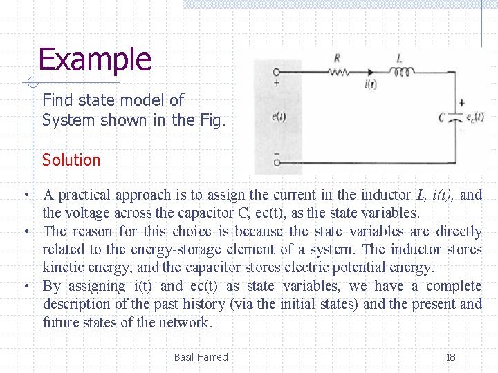
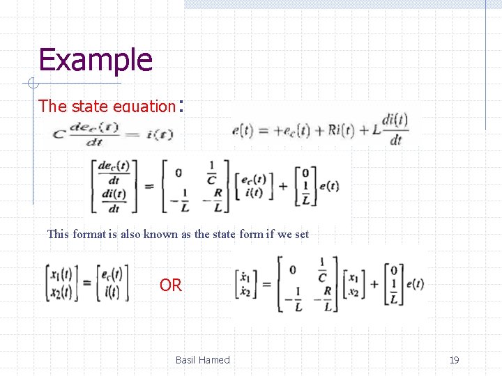
Example Find state model of System shown in the Fig. Solution • A practical approach is to assign the current in the inductor L, i(t), and the voltage across the capacitor C, ec(t), as the state variables. • The reason for this choice is because the state variables are directly related to the energy-storage element of a system. The inductor stores kinetic energy, and the capacitor stores electric potential energy. • By assigning i(t) and ec(t) as state variables, we have a complete description of the past history (via the initial states) and the present and future states of the network. Basil Hamed 18

Example The state equation: This format is also known as the state form if we set OR Basil Hamed 19

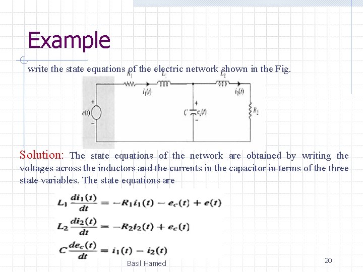
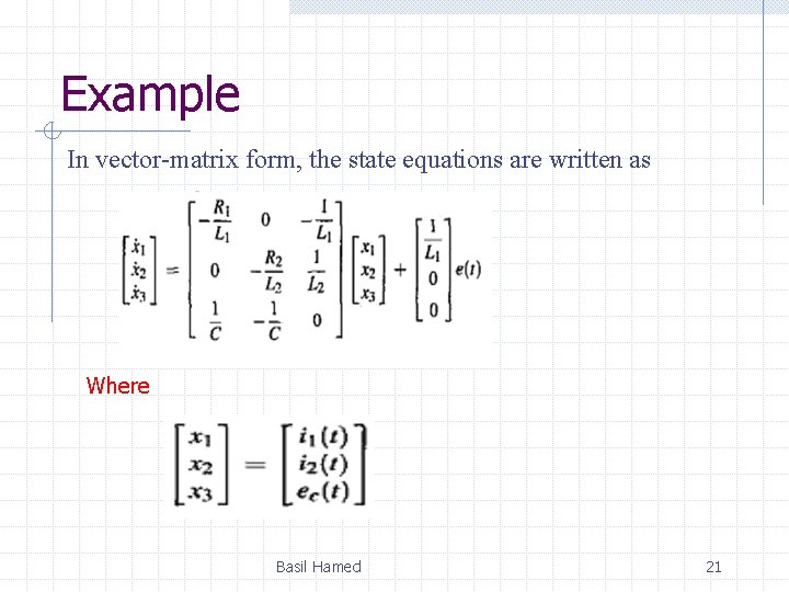
Example write the state equations of the electric network shown in the Fig. Solution: The state equations of the network are obtained by writing the voltages across the inductors and the currents in the capacitor in terms of the three state variables. The state equations are Basil Hamed 20

Example In vector-matrix form, the state equations are written as Where Basil Hamed 21

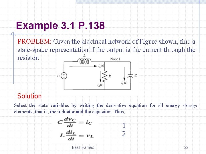
Example 3. 1 P. 138 PROBLEM: Given the electrical network of Figure shown, find a state-space representation if the output is the current through the resistor. Solution Select the state variables by writing the derivative equation for all energy storage elements, that is, the inductor and the capacitor. Thus, 1 2 Basil Hamed 22

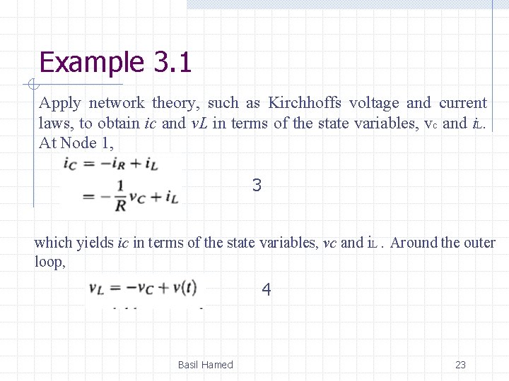
Example 3. 1 Apply network theory, such as Kirchhoffs voltage and current laws, to obtain ic and v. L in terms of the state variables, vc and i. L. At Node 1, 3 which yields ic in terms of the state variables, vc and i. L. Around the outer loop, 4 Basil Hamed 23

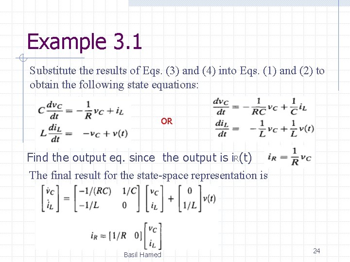
Example 3. 1 Substitute the results of Eqs. (3) and (4) into Eqs. (1) and (2) to obtain the following state equations: OR Find the output eq. since the output is i. R(t) The final result for the state-space representation is Basil Hamed 24

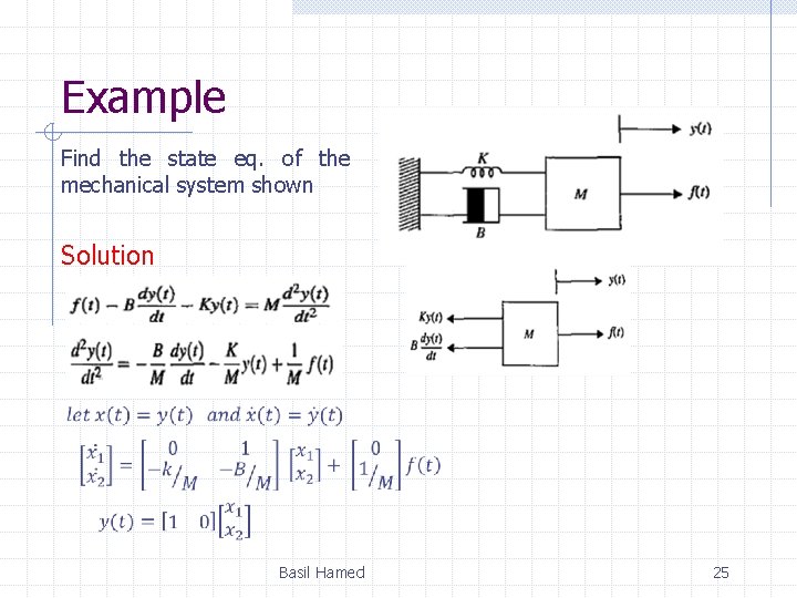
Example Find the state eq. of the mechanical system shown Solution Basil Hamed 25

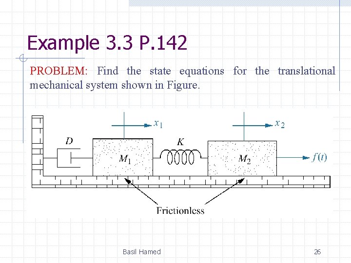
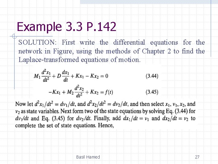
Example 3. 3 P. 142 PROBLEM: Find the state equations for the translational mechanical system shown in Figure. Basil Hamed 26

Example 3. 3 P. 142 SOLUTION: First write the differential equations for the network in Figure, using the methods of Chapter 2 to find the Laplace-transformed equations of motion. Basil Hamed 27

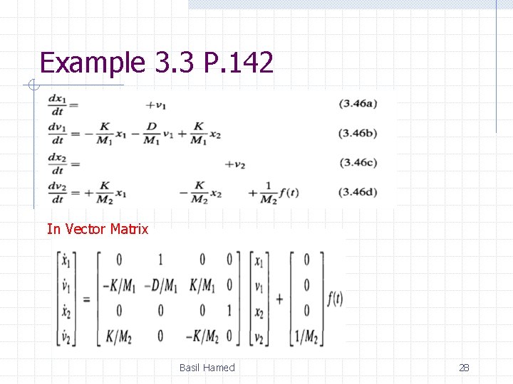
Example 3. 3 P. 142 In Vector Matrix Basil Hamed 28

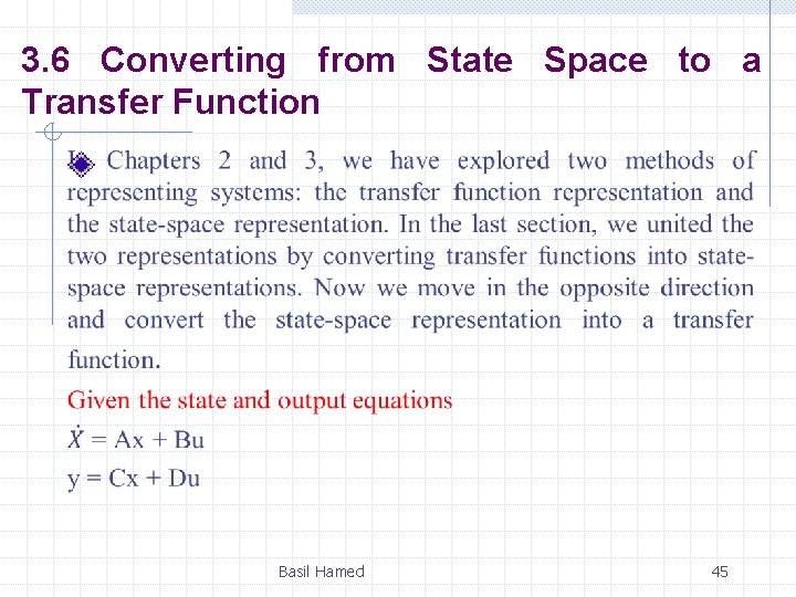
3. 5 Converting a Transfer Function to State Space In the last section, we applied the state-space representation to electrical and mechanical systems. We learn how to convert a transfer function representation to a state-space representation in this section. One advantage of the state-space representation is that it can be used for the simulation of physical systems on the digital computer. Thus, if we want to simulate a system that is represented by a transfer function, we must first convert the transfer function representation to state space. Basil Hamed 29

Converting T. F to S. S • System modeling in state space can take on many representations • Although each of these models yields the same output for a given input, an engineer may prefer a particular one for several reasons. • Another motive for choosing a particular set of state variables and state-space model is ease of solution. Basil Hamed 30

Converting T. F to S. S There are many ways of converting T. F into S. S but the most useful and famous are: 1. Direct Decomposition 2. Cascade Decomposition 3. Parallel Decomposition Basil Hamed 31

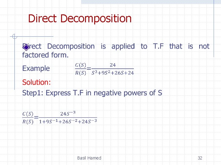
Direct Decomposition Basil Hamed 32

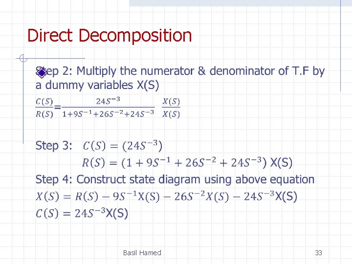
Direct Decomposition Basil Hamed 33

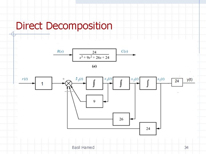
Direct Decomposition Basil Hamed 34

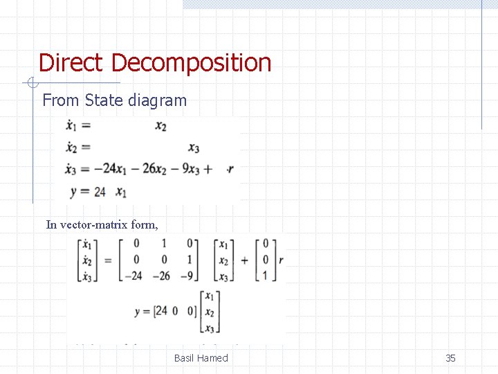
Direct Decomposition From State diagram In vector-matrix form, Basil Hamed 35

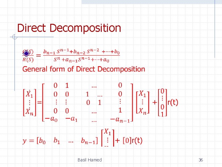
Direct Decomposition Basil Hamed 36

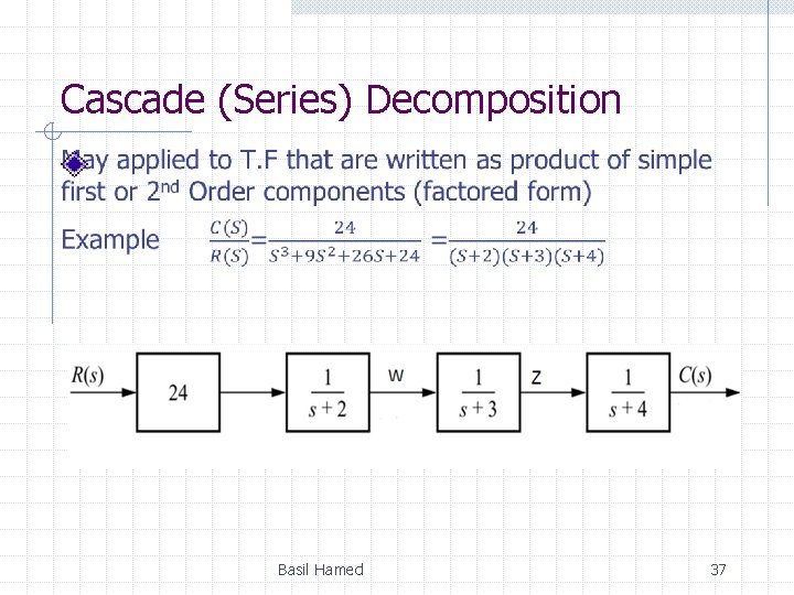
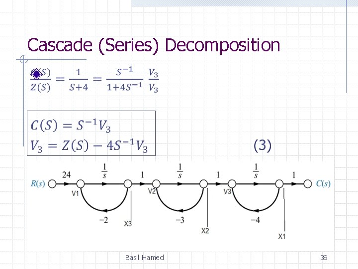
Cascade (Series) Decomposition Basil Hamed 37

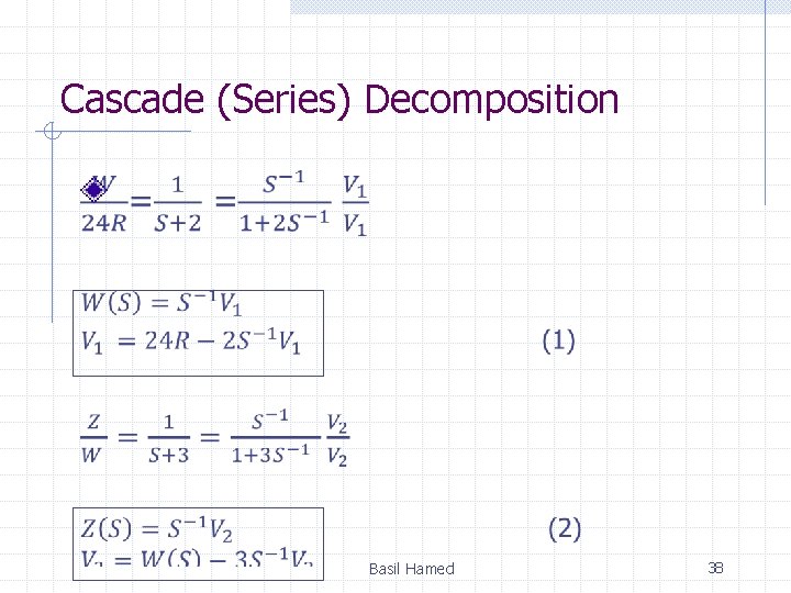
Cascade (Series) Decomposition Basil Hamed 38

Cascade (Series) Decomposition Basil Hamed 39

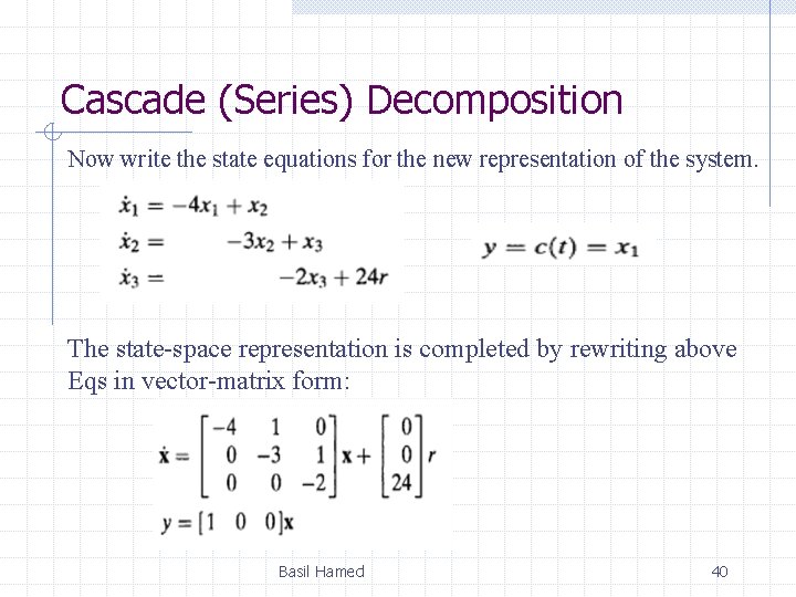
Cascade (Series) Decomposition Now write the state equations for the new representation of the system. The state-space representation is completed by rewriting above Eqs in vector-matrix form: Basil Hamed 40

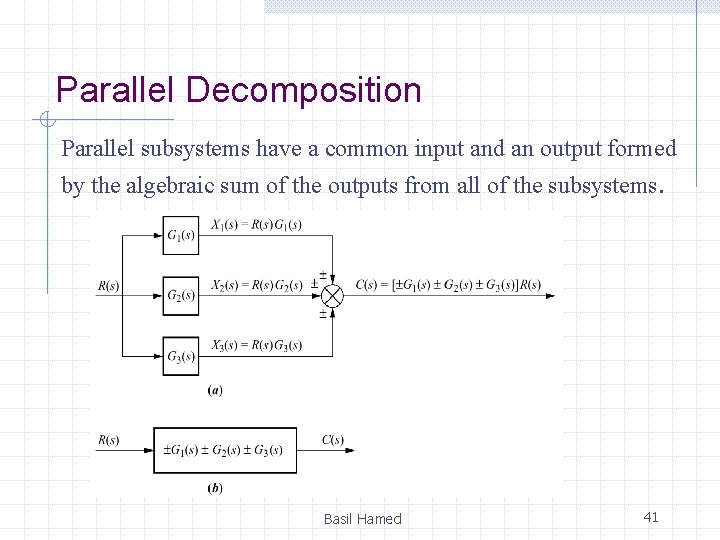
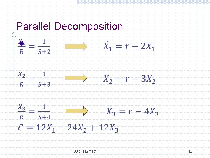
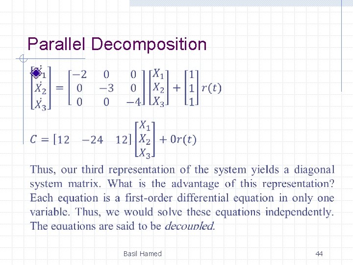
Parallel Decomposition Parallel subsystems have a common input and an output formed by the algebraic sum of the outputs from all of the subsystems. Basil Hamed 41

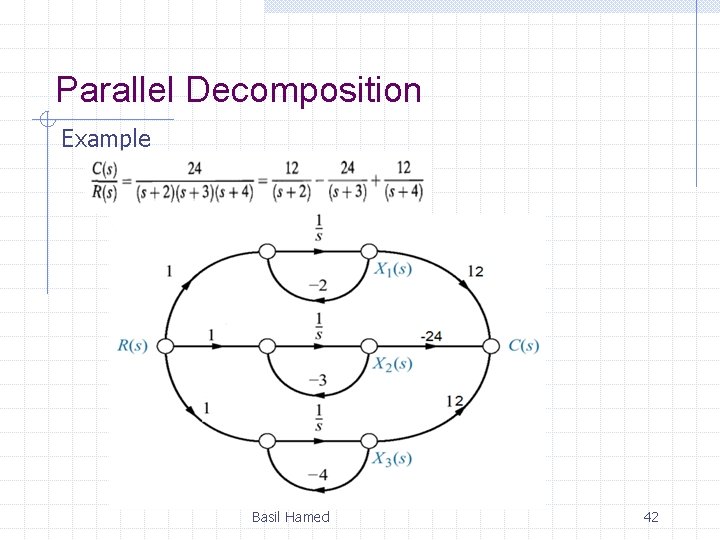
Parallel Decomposition Example Basil Hamed 42

Parallel Decomposition Basil Hamed 43

Parallel Decomposition Basil Hamed 44

3. 6 Converting from State Space to a Transfer Function Basil Hamed 45

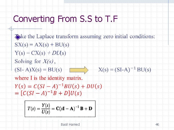
Converting From S. S to T. F Basil Hamed 46

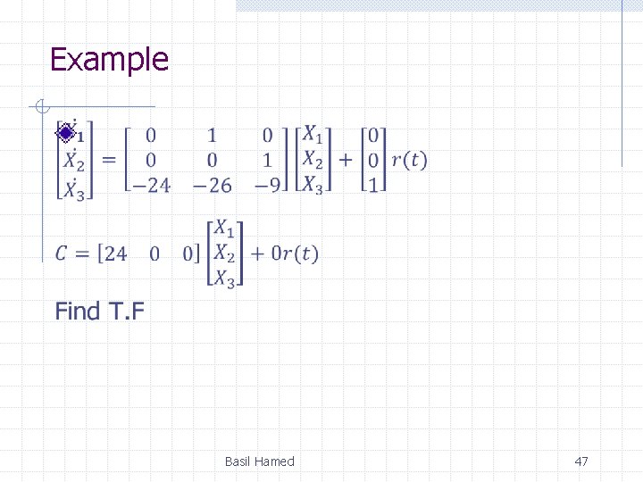
Example Basil Hamed 47

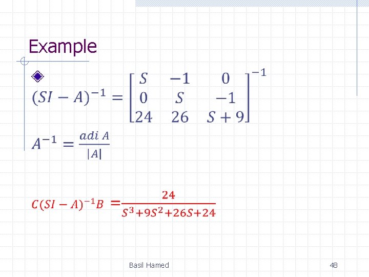
Example Basil Hamed 48

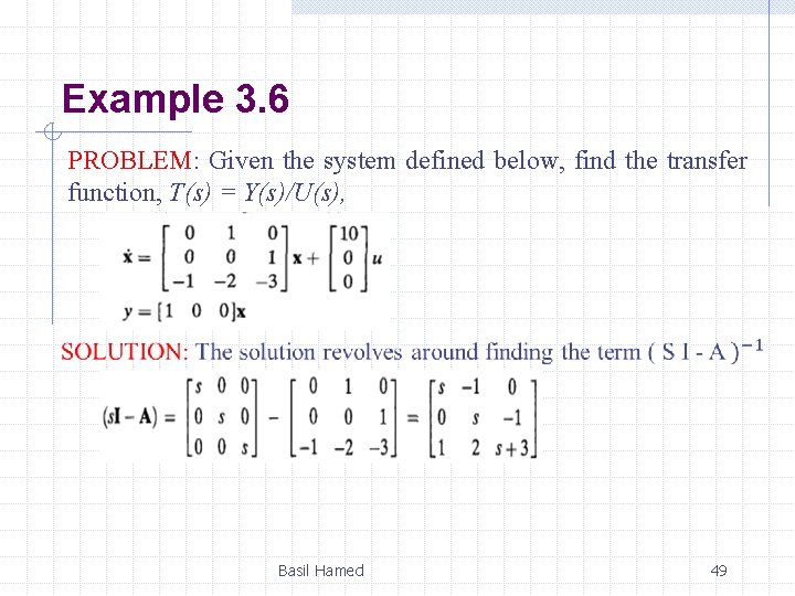
Example 3. 6 PROBLEM: Given the system defined below, find the transfer function, T(s) = Y(s)/U(s), Basil Hamed 49

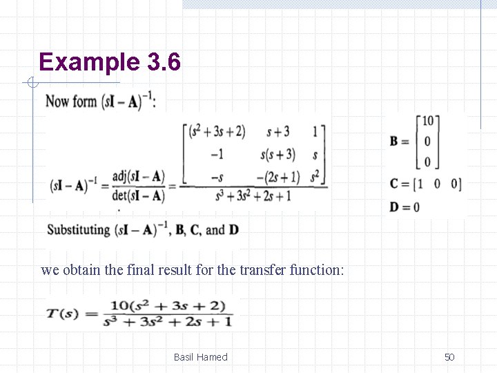
Example 3. 6 we obtain the final result for the transfer function: Basil Hamed 50

3. 7 Linearization • A prime advantage of the state-space representation over the transfer function representation is the ability to represent systems with nonlinearities. • A linearized model is valid only for limited range of operation, and often only at the operating point at which the linearized is carried out. Basil Hamed 51

Why Linearization • Lack of systematic design methodology for direct design of nonlinear control system. • Linear analysis methodology available • The Laplace transform cannot be used to solve nonlinear Diff. EQ. Basil Hamed 52

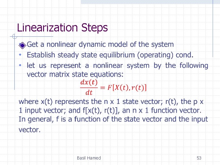
Linearization Steps Basil Hamed 53

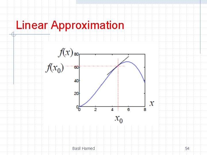
Linear Approximation Basil Hamed 54

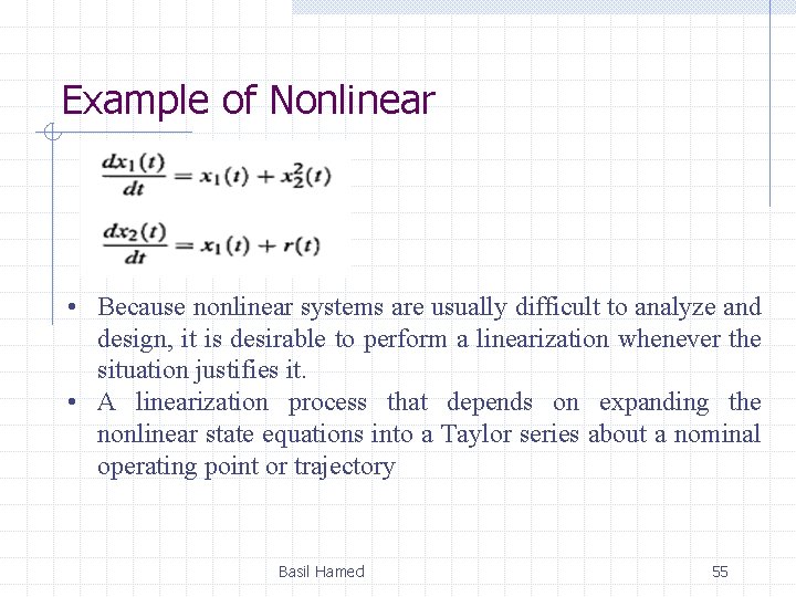
Example of Nonlinear • Because nonlinear systems are usually difficult to analyze and design, it is desirable to perform a linearization whenever the situation justifies it. • A linearization process that depends on expanding the nonlinear state equations into a Taylor series about a nominal operating point or trajectory Basil Hamed 55

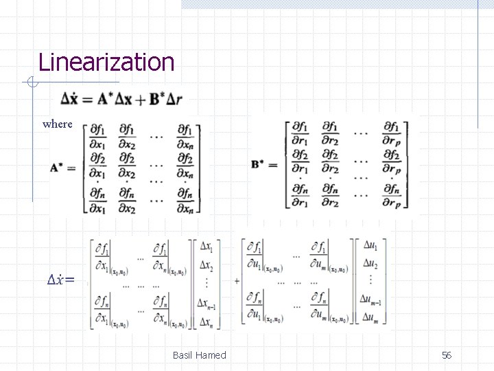
Linearization where Basil Hamed 56

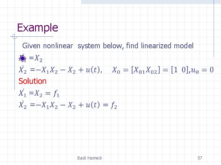
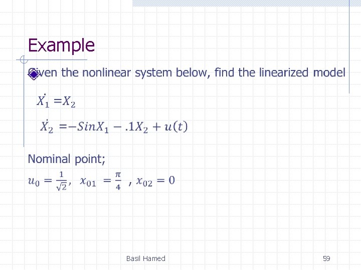
Example Given nonlinear system below, find linearized model Basil Hamed- 57

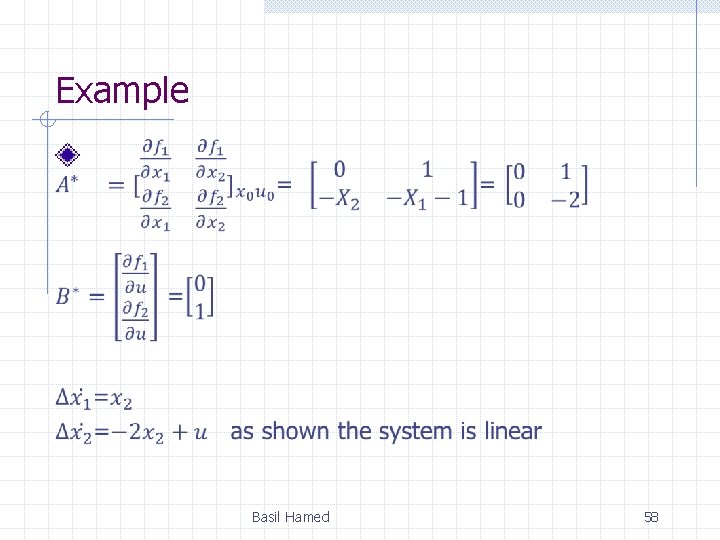
Example Basil Hamed 58

Example Basil Hamed 59

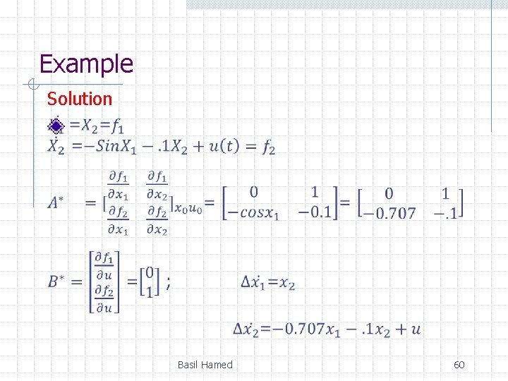
Example Solution Basil Hamed 60

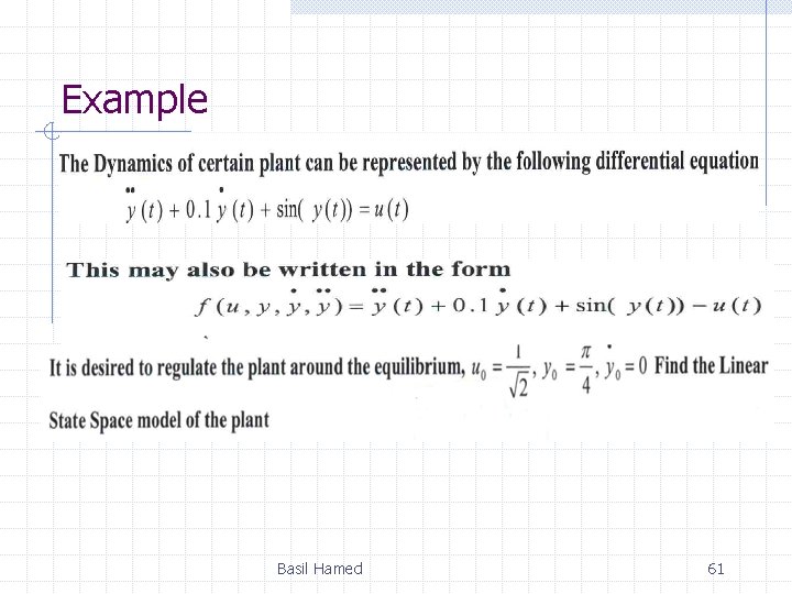
Example Basil Hamed 61

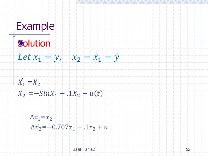
Example Basil Hamed 62

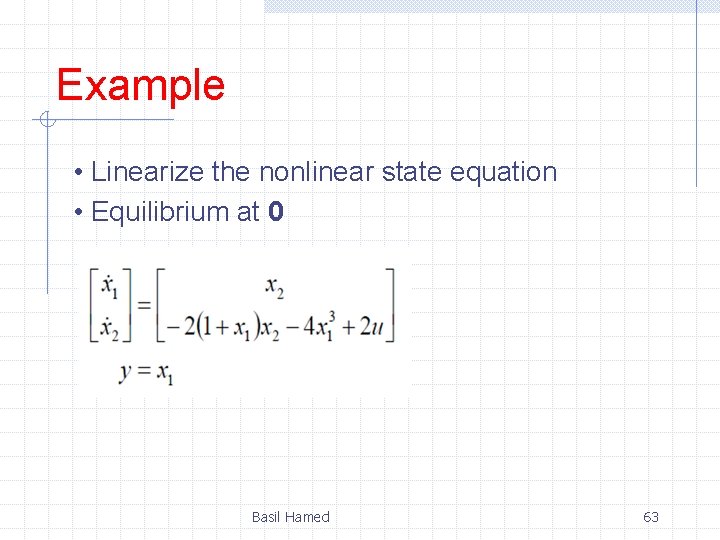
Example • Linearize the nonlinear state equation • Equilibrium at 0 Basil Hamed 63

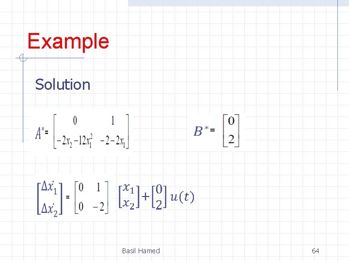
Example Solution Basil Hamed 64