Control System Specifications Purpose to quantify a good

Control System Specifications • Purpose: to quantify a good control system • Metrics or specifications: – From input/output response point of view • Time domain – Initial responsiveness, response time – Transition behavior, overshoot – Final settling, settling time, settling accuracy • Frequency domain – Bandwidth, crossover frequencies – Resonance, margins – Low frequency gain – From a stability point of view • Stable, no bad poles • Pole locations, distance to jw-axis, angle to real axis • Pole movement direction and sensitivity, as system parameter varies

Dynamic Response • Steady State Response: the part of response when t → ∞ • Transient response: the part of response right after the input is being applied. • Both are part of the total response total resp = z. i. resp + z. s. resp. z. i. resp = “Output due to i. c. when input ≡ 0” z. s. resp = “Output due to input excitation when all i. c. are set=0 at t=0” Both z. i. resp and z. s. resp have their own transient resp and their own steady state resp. Here ignore i. c. and consider z. s. resp.

Typical test signal • Unit step signal: us(t) 1 0 • Unit impulse: δ(t) t

• Unit ramp: r(t) t • Unit acc. signal: a(t) 0. 5 0 1 t

• Exponential signal: 1 0 • One sided sinusoidal: t

• Unit step response: u(s)= 1 y(s)=H(s) s In Matlab: step(sys) • Unit impulse resp: u(s)=1 Matlab: impulse(sys) H(s) y(s)=H(s) 1 s

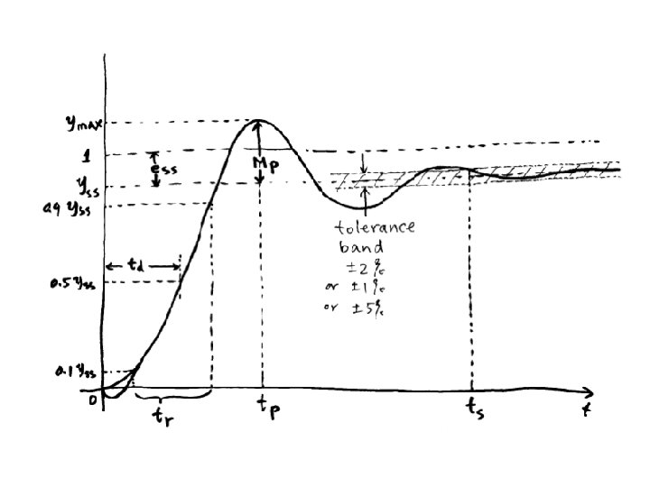
Time domain response specifications • Defined based on unit step response • Defined for closed-loop system • Steady-state value yss • Steady-state error ess • Settling time ts = time when y(t) last enters a tolerance band

If yss = 1 tp

Step response is: By final value theorem In MATLAB: num = [. . . . ]; den=[……]; b 0 = num(length(num)), or num(end) a 0 = den(length(den)), or den(end) yss=b 0/a 0

If numerical values of y and t available, from [y, t] = step(num, den); abs(y – yss) < tol means inside band abs(y – yss) ≥ tol not inside e. g. t_out = t(abs(y – yss) >= tol) contains all those time points when y is not inside the band. Therefore, the last value in t_out will be the settling time. ts=t_out(end)

Peak time tp = time when y(t) reaches its maximum value. Peak value ymax = y(tp) Hence: ymax = max(y); tp = t(y == ymax); Overshoot: OS = ymax - yss Percentage overshoot: If ymax =y(end) no overshoot no tp

If t 50 = t(y >= 0. 5*yss), this contains all time points when y(t) is ≥ 50% of yss so the first such point is td. td = t 50(1); Similarly, t 10 = t(y <= 0. 1*yss) & t 90 = t(y >= 0. 9*yss) can be used to find tr. tr = t 90(1) – t 10(end)

90%yss 10%yss tr≈0. 45 ts td≈0. 35 tp≈0. 9 sec

If you use tp = t(y==max(y)), you get tp = 1. 5; to fix this, set tp=inf if tp==t(end) ts=0. 45 yss=1 ess=0 O. S. =0 Mp=0 tp=∞ td≈0. 2 tr≈0. 35

tp=0. 35 ts≈0. 92 O. S. =0. 4 Mp=40% yss=1 ess=0 td≈0. 2 tr≈0. 1

Transient Response • First order system transient response – Step response specs and relationship to pole location • Second order system transient response – Step response specs and relationship to pole location • Effects of additional poles and zeros

Prototype first order system E U(s) + - 1 τs Y(s)

First order system step resp Normalized time t/t

Prototype first order system • • • No overshoot, tp=inf, Mp = 0 Yss=1, ess=0 Settling time ts = [-ln(tol)]/p Delay time td = [-ln(0. 5)]/p Rise time tr = [ln(0. 9) – ln(0. 1)]/p • All times proportional to 1/p= t • Larger p means faster response

The error signal: e(t) = 1 -y(t)=e-ptus(t) Normalized time t/t

In every τ seconds, the error is reduced by 63. 2%

General First-order system We know how this responds to input Step response starts at y(0+)=k, final value kz/p 1/p = t is still time constant; After 0+, in every t, y(t) moves 63. 2% closer to final value

Step response by MATLAB: >> p =. . >> n = [ b 1 b 0 ] >> d = [ 1 p ] >> step ( n , d ) Other MATLAB commands to explore: plot, hold, axis, xlabel, ylabel, title, text, gtext, semilogx, semilogy, loglog, subplot

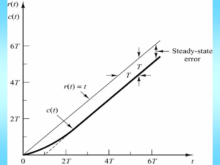
Unit ramp response:

Note: In step response, the steady-state tracking error = zero.

Unit impulse response: