Control structure design What should we measure control

Control structure design: What should we measure, control and manipulate? Sigurd Skogestad Department of Chemical Engineering NTNU, Trondheim First African Control Conference, Cape Town, 04 December 2003 1

Outline • • • 2 About myself Control structure design A procedure for control structure design Selection of primary controlled variables Example stabilizing control: Anti slug control Conclusion

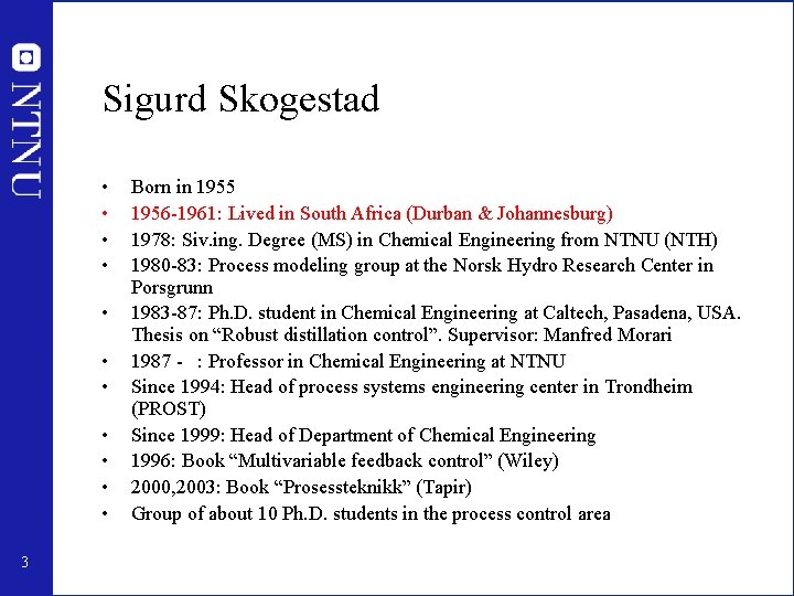
Sigurd Skogestad • • • 3 Born in 1955 1956 -1961: Lived in South Africa (Durban & Johannesburg) 1978: Siv. ing. Degree (MS) in Chemical Engineering from NTNU (NTH) 1980 -83: Process modeling group at the Norsk Hydro Research Center in Porsgrunn 1983 -87: Ph. D. student in Chemical Engineering at Caltech, Pasadena, USA. Thesis on “Robust distillation control”. Supervisor: Manfred Morari 1987 - : Professor in Chemical Engineering at NTNU Since 1994: Head of process systems engineering center in Trondheim (PROST) Since 1999: Head of Department of Chemical Engineering 1996: Book “Multivariable feedback control” (Wiley) 2000, 2003: Book “Prosessteknikk” (Tapir) Group of about 10 Ph. D. students in the process control area

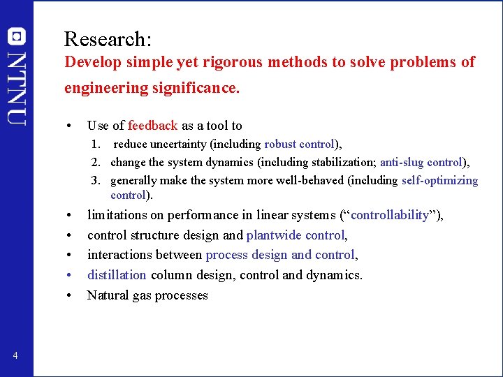
Research: Develop simple yet rigorous methods to solve problems of engineering significance. • Use of feedback as a tool to 1. reduce uncertainty (including robust control), 2. change the system dynamics (including stabilization; anti-slug control), 3. generally make the system more well-behaved (including self-optimizing control). • • • 4 limitations on performance in linear systems (“controllability”), control structure design and plantwide control, interactions between process design and control, distillation column design, control and dynamics. Natural gas processes

Outline • • • 5 About myself Control structure design A procedure for control structure design Selection of primary controlled variables Example stabilizing control: Anti slug control Conclusion

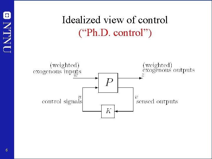
Idealized view of control (“Ph. D. control”) 6

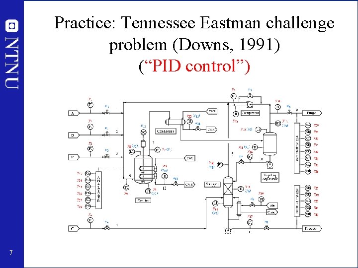
Practice: Tennessee Eastman challenge problem (Downs, 1991) (“PID control”) 7

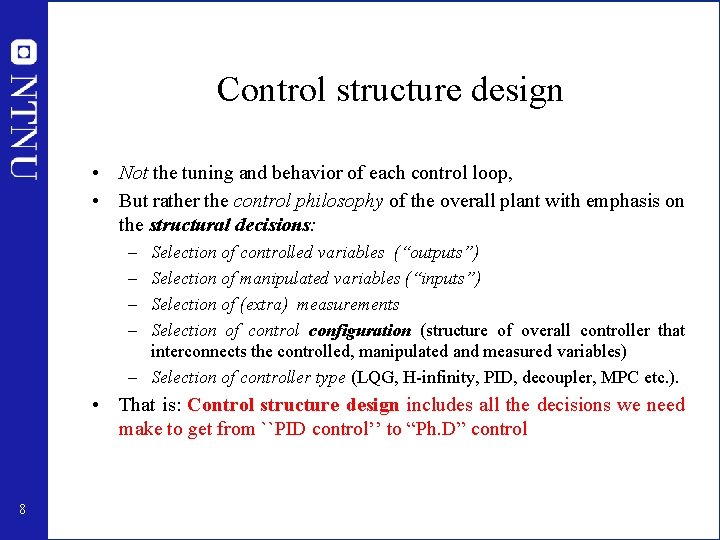
Control structure design • Not the tuning and behavior of each control loop, • But rather the control philosophy of the overall plant with emphasis on the structural decisions: – – Selection of controlled variables (“outputs”) Selection of manipulated variables (“inputs”) Selection of (extra) measurements Selection of control configuration (structure of overall controller that interconnects the controlled, manipulated and measured variables) – Selection of controller type (LQG, H-infinity, PID, decoupler, MPC etc. ). • That is: Control structure design includes all the decisions we need make to get from ``PID control’’ to “Ph. D” control 8

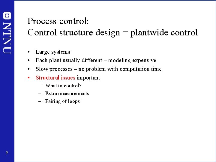
Process control: Control structure design = plantwide control • • Large systems Each plant usually different – modeling expensive Slow processes – no problem with computation time Structural issues important – What to control? – Extra measurements – Pairing of loops 9

• Control structure selection issues are identified as important also in other industries. Professor Gary Balas at ECC’ 03 about flight control at Boeing: The most important control issue has always been to select the right controlled variables --- no systematic tools used! 10

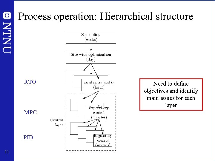
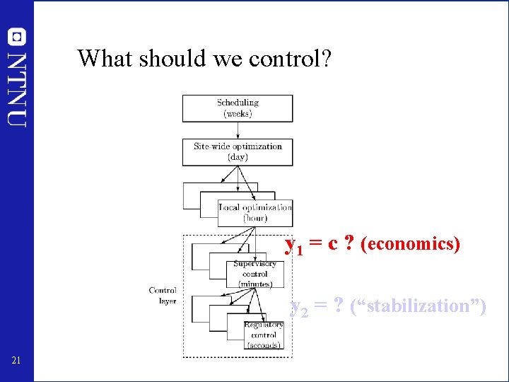
Process operation: Hierarchical structure RTO MPC PID 11 Need to define objectives and identify main issues for each layer

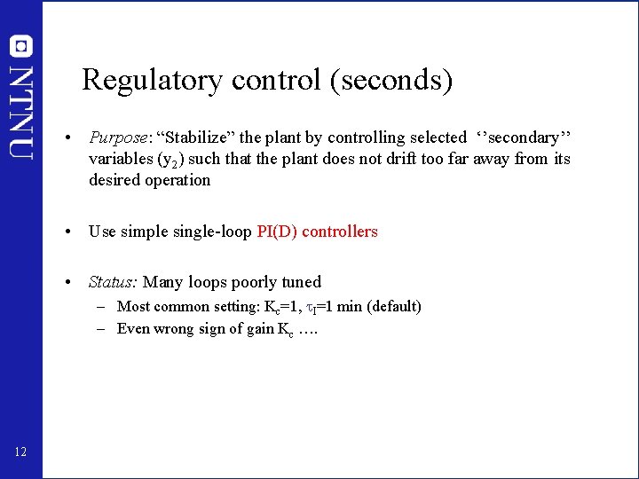
Regulatory control (seconds) • Purpose: “Stabilize” the plant by controlling selected ‘’secondary’’ variables (y 2) such that the plant does not drift too far away from its desired operation • Use simple single-loop PI(D) controllers • Status: Many loops poorly tuned – Most common setting: Kc=1, I=1 min (default) – Even wrong sign of gain Kc …. 12

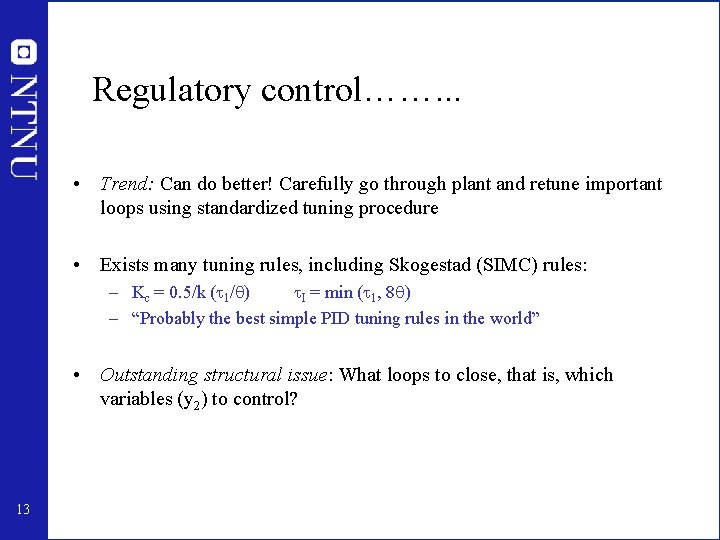
Regulatory control……. . . • Trend: Can do better! Carefully go through plant and retune important loops using standardized tuning procedure • Exists many tuning rules, including Skogestad (SIMC) rules: – Kc = 0. 5/k ( 1/ ) I = min ( 1, 8 ) – “Probably the best simple PID tuning rules in the world” • Outstanding structural issue: What loops to close, that is, which variables (y 2) to control? 13

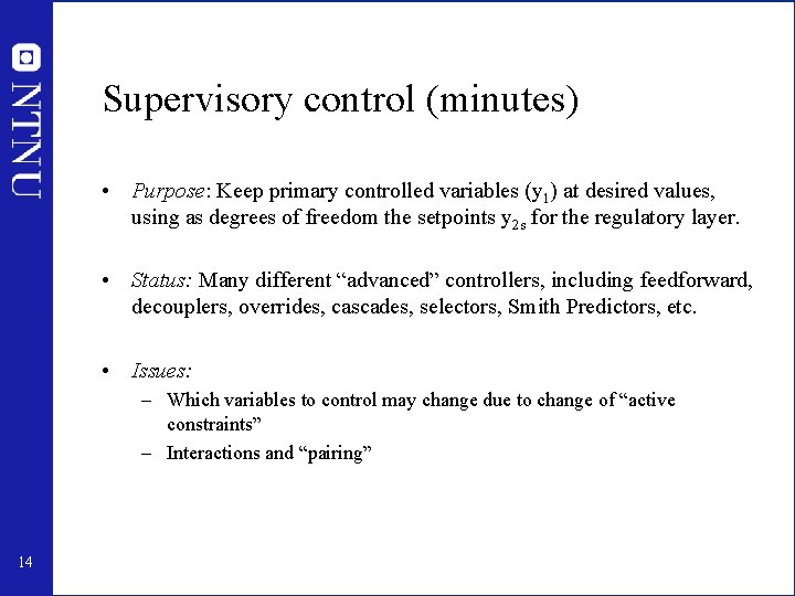
Supervisory control (minutes) • Purpose: Keep primary controlled variables (y 1) at desired values, using as degrees of freedom the setpoints y 2 s for the regulatory layer. • Status: Many different “advanced” controllers, including feedforward, decouplers, overrides, cascades, selectors, Smith Predictors, etc. • Issues: – Which variables to control may change due to change of “active constraints” – Interactions and “pairing” 14

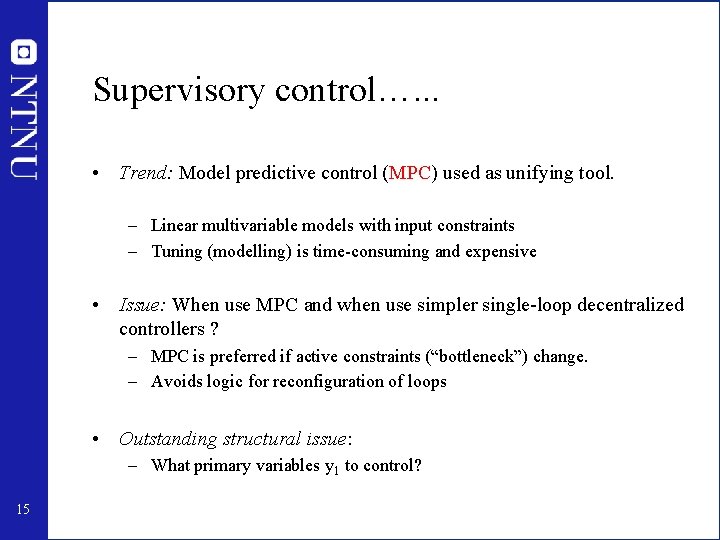
Supervisory control…. . . • Trend: Model predictive control (MPC) used as unifying tool. – Linear multivariable models with input constraints – Tuning (modelling) is time-consuming and expensive • Issue: When use MPC and when use simpler single-loop decentralized controllers ? – MPC is preferred if active constraints (“bottleneck”) change. – Avoids logic for reconfiguration of loops • Outstanding structural issue: – What primary variables y 1 to control? 15

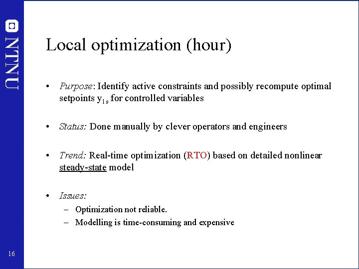
Local optimization (hour) • Purpose: Identify active constraints and possibly recompute optimal setpoints y 1 s for controlled variables • Status: Done manually by clever operators and engineers • Trend: Real-time optimization (RTO) based on detailed nonlinear steady-state model • Issues: – Optimization not reliable. – Modelling is time-consuming and expensive 16

Outline • • • 17 About myself Control structure design A procedure for control structure design Selection of primary controlled variables Example stabilizing control: Anti slug control Conclusion

Stepwise procedure plantwide control I. TOP-DOWN Step 1. DEFN. OF OPERATIONAL OBJECTIVES Step 2. MANIPULATED VARIABLES and DEGREE OF FREEDOM ANALYSIS Step 3. WHAT TO CONTROL? (primary outputs, c= y 1) Step 4. PRODUCTION RATE 18

II. BOTTOM-UP (structure control system): Step 5. REGULATORY CONTROL LAYER Stabilization and Local disturbance rejection What more to control? (secondary outputs y 2) Step 6. SUPERVISORY CONTROL LAYER Decentralized control or MPC? Step 7. OPTIMIZATION LAYER (RTO) 19

Outline • • • 20 About myself Control structure design A procedure for control structure design Selection of primary controlled variables Example stabilizing control: Anti slug control Conclusion

What should we control? y 1 = c ? (economics) y 2 = ? (“stabilization”) 21

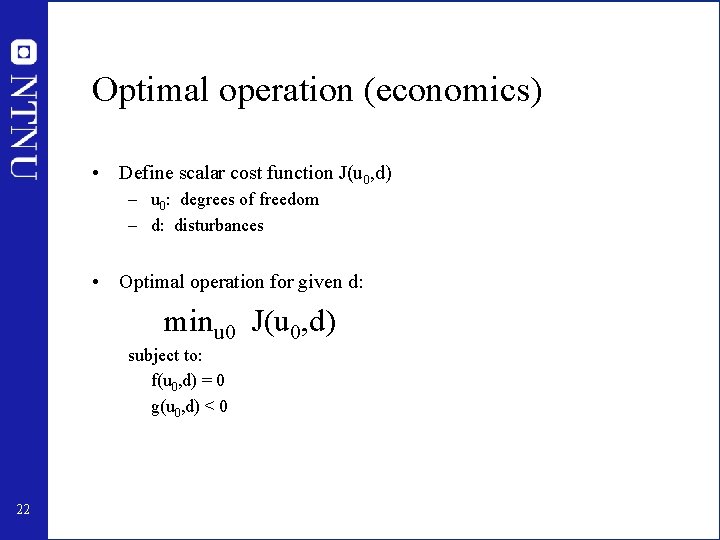
Optimal operation (economics) • Define scalar cost function J(u 0, d) – u 0: degrees of freedom – d: disturbances • Optimal operation for given d: minu 0 J(u 0, d) subject to: f(u 0, d) = 0 g(u 0, d) < 0 22

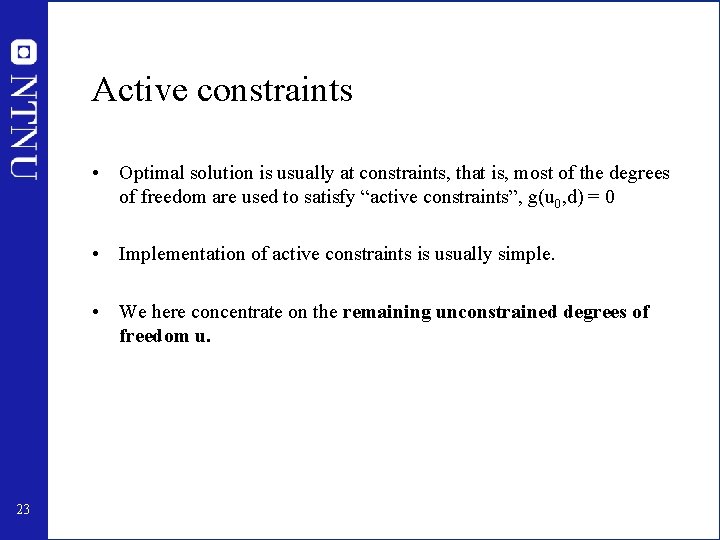
Active constraints • Optimal solution is usually at constraints, that is, most of the degrees of freedom are used to satisfy “active constraints”, g(u 0, d) = 0 • Implementation of active constraints is usually simple. • We here concentrate on the remaining unconstrained degrees of freedom u. 23

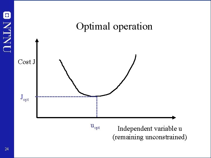
Optimal operation Cost J Jopt uopt 24 Independent variable u (remaining unconstrained)

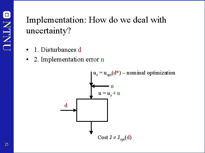
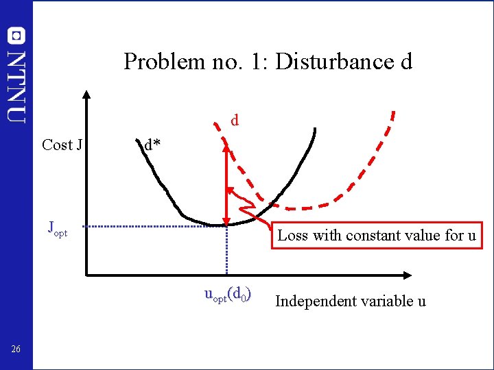
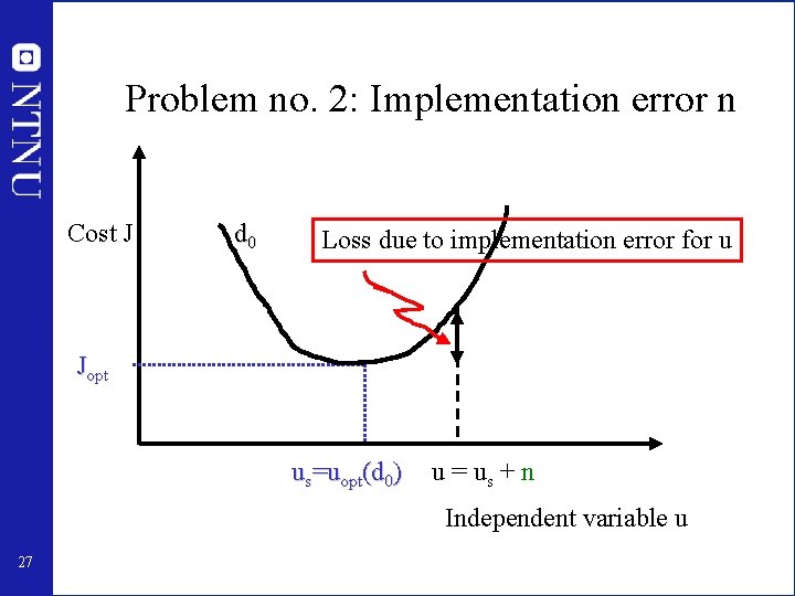
Implementation: How do we deal with uncertainty? • 1. Disturbances d • 2. Implementation error n us = uopt(d*) – nominal optimization n u = us + n d Cost J Jopt(d) 25

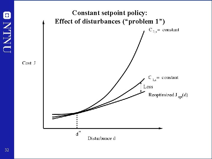
Problem no. 1: Disturbance d d Cost J d* Jopt Loss with constant value for u uopt(d 0) 26 Independent variable u

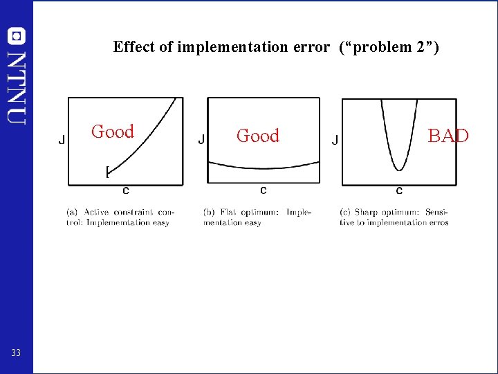
Problem no. 2: Implementation error n Cost J d 0 Loss due to implementation error for u Jopt us=uopt(d 0) u = us + n Independent variable u 27

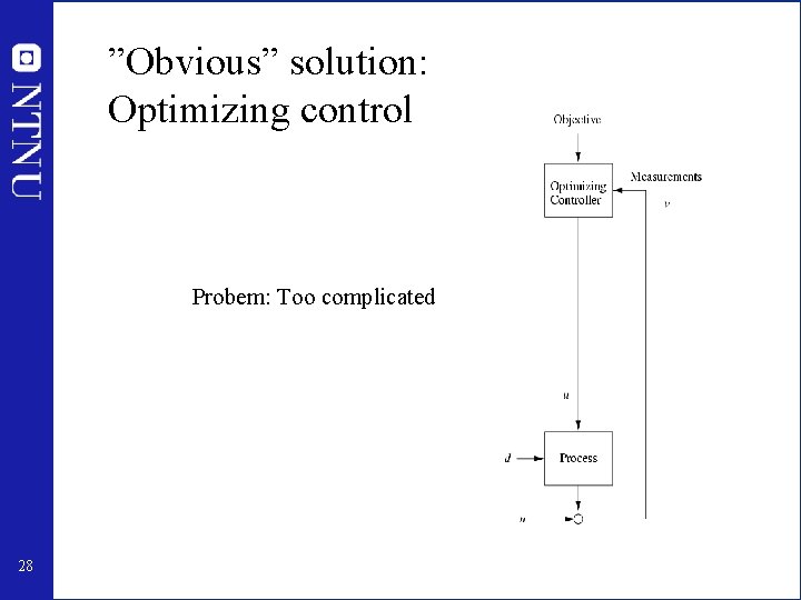
”Obvious” solution: Optimizing control Probem: Too complicated 28

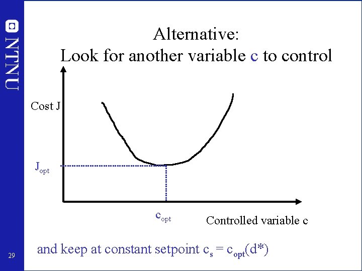
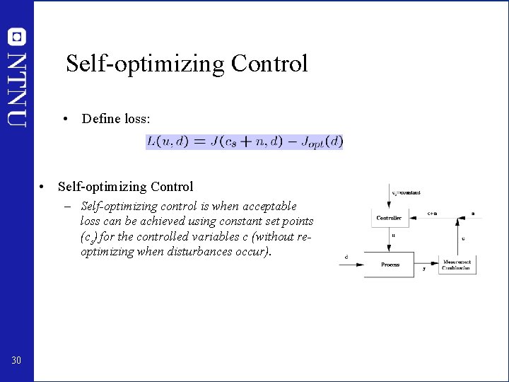
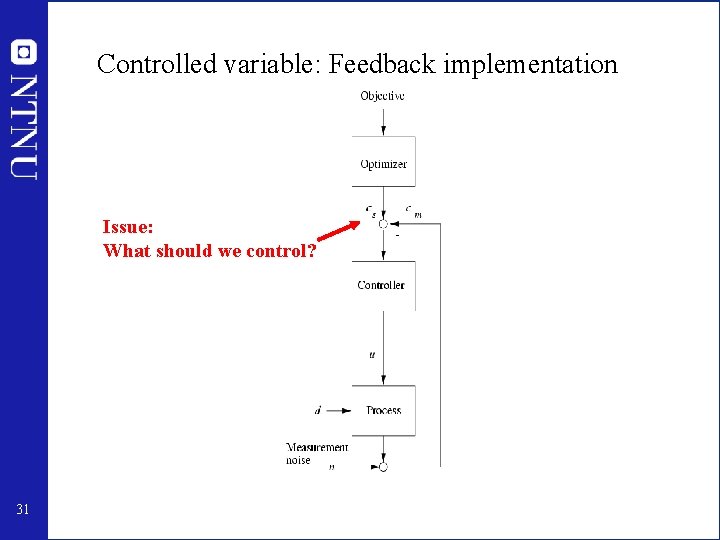
Alternative: Look for another variable c to control Cost J Jopt copt 29 Controlled variable c and keep at constant setpoint cs = copt(d*)

Self-optimizing Control • Define loss: • Self-optimizing Control – Self-optimizing control is when acceptable loss can be achieved using constant set points (cs) for the controlled variables c (without reoptimizing when disturbances occur). 30

Controlled variable: Feedback implementation Issue: What should we control? 31

Constant setpoint policy: Effect of disturbances (“problem 1”) 32

Effect of implementation error (“problem 2”) Good 33 Good BAD

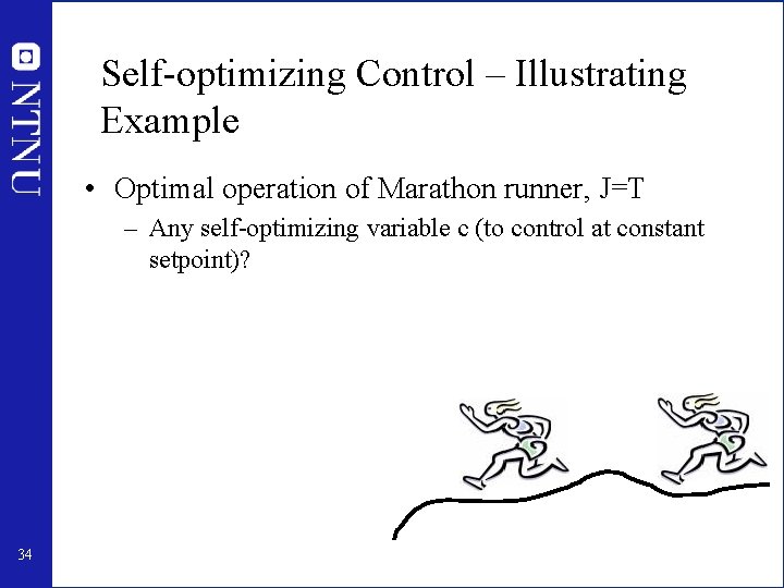
Self-optimizing Control – Illustrating Example • Optimal operation of Marathon runner, J=T – Any self-optimizing variable c (to control at constant setpoint)? 34

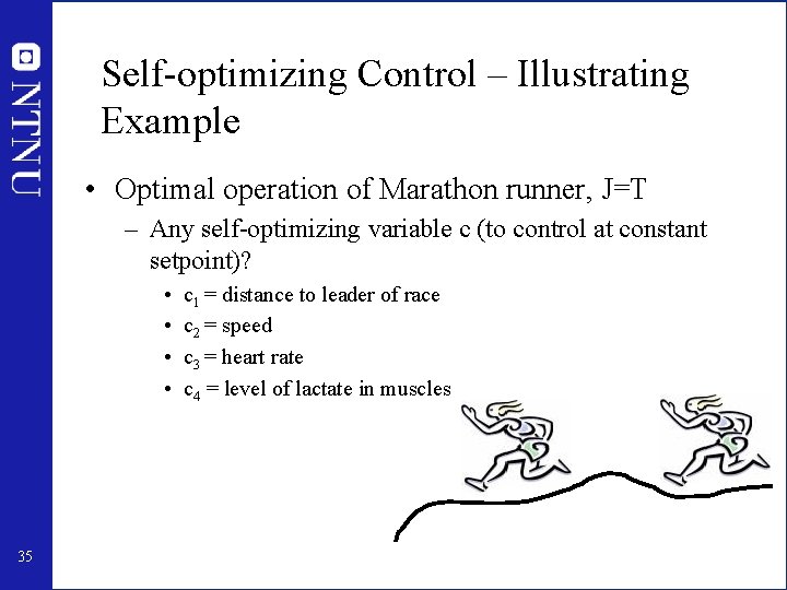
Self-optimizing Control – Illustrating Example • Optimal operation of Marathon runner, J=T – Any self-optimizing variable c (to control at constant setpoint)? • • 35 c 1 = distance to leader of race c 2 = speed c 3 = heart rate c 4 = level of lactate in muscles

Further examples • • 36 Central bank. J = welfare. c=inflation rate Cake baking. J = nice taste, c = Temperature Biology. J = ? , c = regulatory mechanism Business, J = profit. c = KPI = response time to order

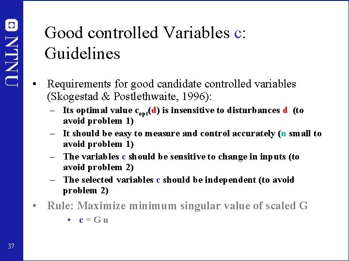
Good controlled Variables c: Guidelines • Requirements for good candidate controlled variables (Skogestad & Postlethwaite, 1996): – Its optimal value copt(d) is insensitive to disturbances d (to avoid problem 1) – It should be easy to measure and control accurately (n small to avoid problem 1) – The variables c should be sensitive to change in inputs (to avoid problem 2) – The selected variables c should be independent (to avoid problem 2) • Rule: Maximize minimum singular value of scaled G • c=Gu 37

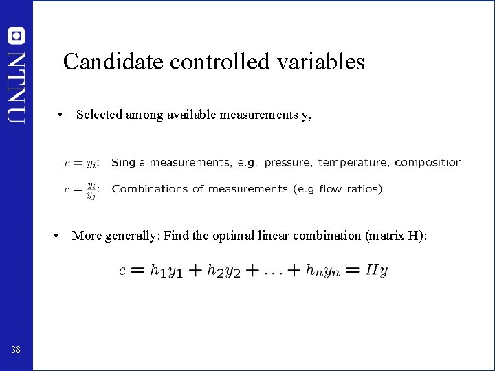
Candidate controlled variables • Selected among available measurements y, • More generally: Find the optimal linear combination (matrix H): 38

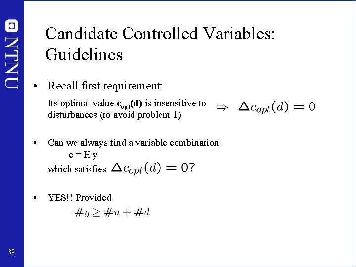
Candidate Controlled Variables: Guidelines • Recall first requirement: Its optimal value copt(d) is insensitive to disturbances (to avoid problem 1) 39 • Can we always find a variable combination c=Hy which satisfies • YES!! Provided

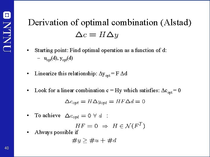
Derivation of optimal combination (Alstad) • Starting point: Find optimal operation as a function of d: – uopt(d), yopt(d) • Linearize this relationship: yopt = F d • Look for a linear combination c = Hy which satisfies: copt = 0 • To achieve • Always possible if 40

Applications of self-optimizing control • • 41 Distillation Tennessee Eastman Challenge problem Power plant +++

Outline • • • 42 About myself Control structure design A procedure for control structure design Selection of primary controlled variables Example stabilizing control: Anti-slug control Conclusion

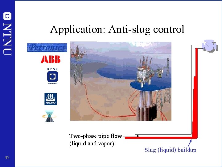
Application: Anti-slug control Two-phase pipe flow (liquid and vapor) 43 Slug (liquid) buildup

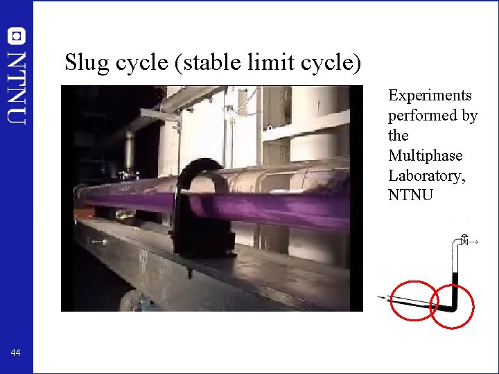
Slug cycle (stable limit cycle) Experiments performed by the Multiphase Laboratory, NTNU 44

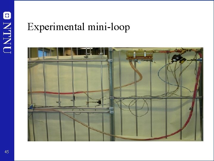
Experimental mini-loop 45

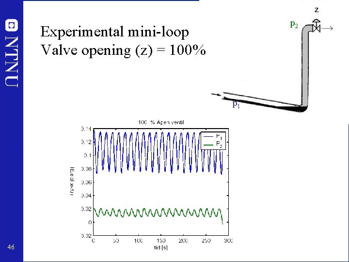
z p 2 Experimental mini-loop Valve opening (z) = 100% p 1 46

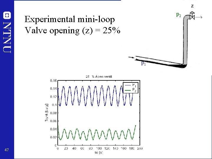
z p 2 Experimental mini-loop Valve opening (z) = 25% p 1 47

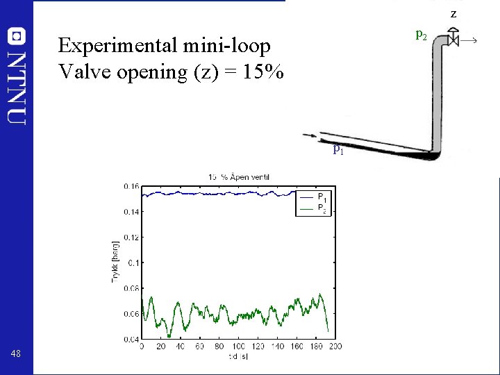
z p 2 Experimental mini-loop Valve opening (z) = 15% p 1 48

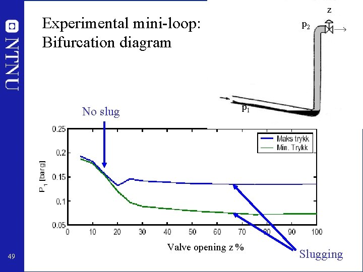
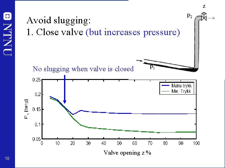
z Experimental mini-loop: Bifurcation diagram No slug p 2 p 1 Valve opening z % 49 Slugging

z Avoid slugging: 1. Close valve (but increases pressure) No slugging when valve is closed p 1 Valve opening z % 50 p 2

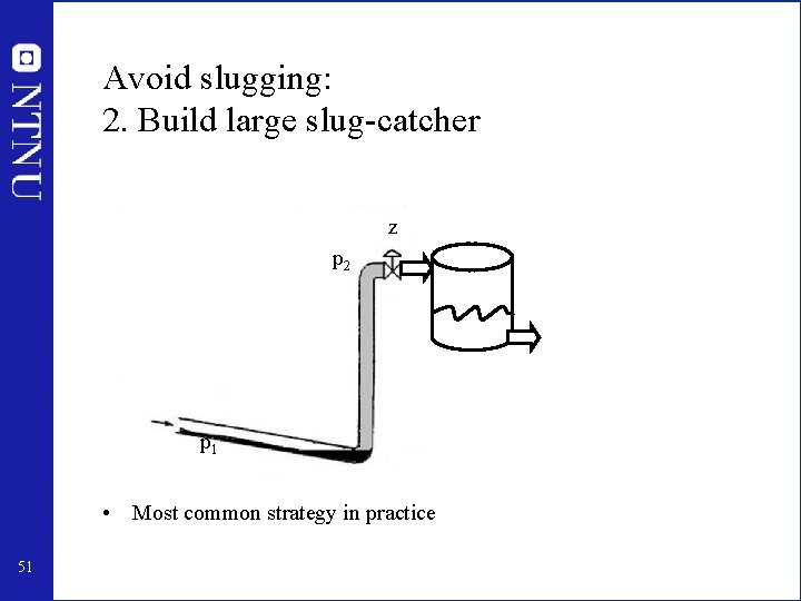
Avoid slugging: 2. Build large slug-catcher z p 2 p 1 • Most common strategy in practice 51

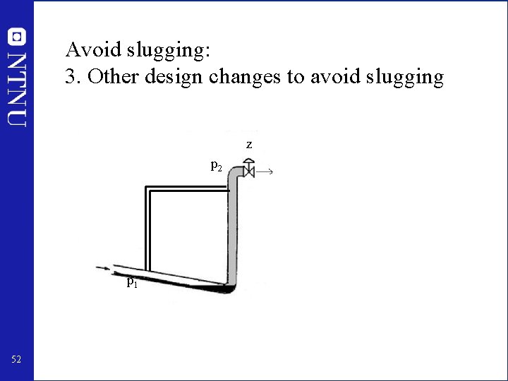
Avoid slugging: 3. Other design changes to avoid slugging z p 2 p 1 52

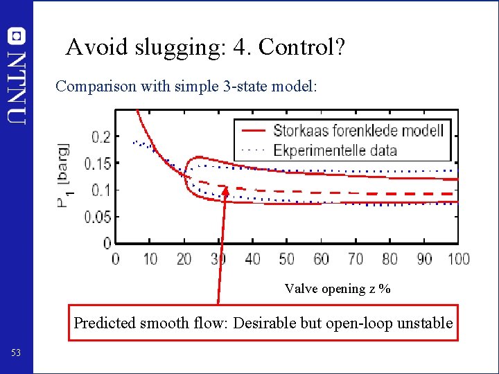
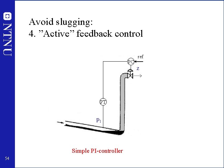
Avoid slugging: 4. Control? Comparison with simple 3 -state model: Valve opening z % Predicted smooth flow: Desirable but open-loop unstable 53

Avoid slugging: 4. ”Active” feedback control PC PT p 1 Simple PI-controller 54 ref z

Anti slug control: Mini-loop experiments p 1 [bar] z [%] 55 Controller ON Controller OFF

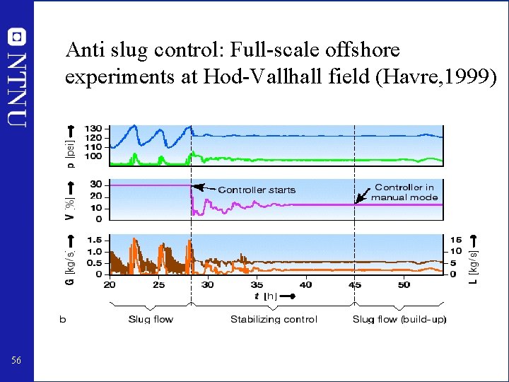
Anti slug control: Full-scale offshore experiments at Hod-Vallhall field (Havre, 1999) 56

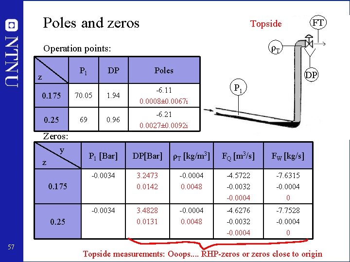
Poles and zeros Topside ρT Operation points: P 1 z FT DP Poles DP 0. 175 70. 05 1. 94 -6. 11 0. 0008± 0. 0067 i 0. 25 69 0. 96 -6. 21 0. 0027± 0. 0092 i P 1 Zeros: y z P 1 [Bar] DP[Bar] ρT [kg/m 3] FQ [m 3/s] FW [kg/s] -0. 0034 3. 2473 0. 0142 -0. 0004 0. 0048 -4. 5722 -0. 0032 -0. 0004 -7. 6315 -0. 0004 0 -0. 0034 3. 4828 0. 0131 -0. 0004 0. 0048 -4. 6276 -0. 0032 -0. 0004 -7. 7528 -0. 0004 0 0. 175 0. 25 57 Topside measurements: Ooops. . RHP-zeros or zeros close to origin

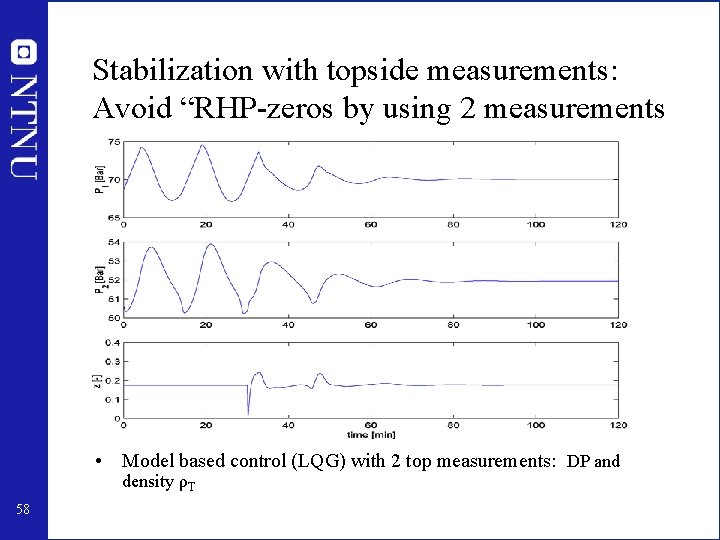
Stabilization with topside measurements: Avoid “RHP-zeros by using 2 measurements • Model based control (LQG) with 2 top measurements: DP and density ρT 58

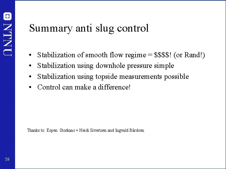
Summary anti slug control • • Stabilization of smooth flow regime = $$$$! (or Rand!) Stabilization using downhole pressure simple Stabilization using topside measurements possible Control can make a difference! Thanks to: Espen Storkaas + Heidi Sivertsen and Ingvald Bårdsen 59

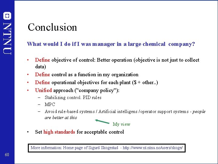
Conclusion What would I do if I was manager in a large chemical company? • • Define objective of control: Better operation (objective is not just to collect data) Define control as a function in my organization Define operational objectives for each plant ($ + other. . ) Unified approach (”company policy”): – Stabilizing control. PID rules – MPC – Avoid rule-based systems / Artificial intelligens /operator support systems - people are better at this My view • Set high standards for acceptable control More information: Home page of Sigurd Skogestad - http: //www. ntnu. no/users/skoge/ 60