Control Loop Interaction CSE 425 Industrial Process Control

Control Loop Interaction CSE 425 Industrial Process Control Lecture 10 1

MIMO systems • Thus far, we have focused on systems with single controlled variable and single manipulated variable. • These are called single-input single-output (SISO) systems. • Most processes, however, are MIMO. 2

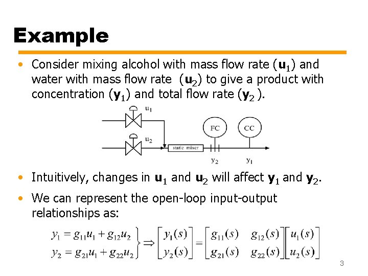
Example • Consider mixing alcohol with mass flow rate (u 1) and water with mass flow rate (u 2) to give a product with concentration (y 1) and total flow rate (y 2 ). • Intuitively, changes in u 1 and u 2 will affect y 1 and y 2. • We can represent the open-loop input-output relationships as: 3

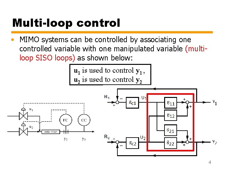
Multi-loop control • MIMO systems can be controlled by associating one controlled variable with one manipulated variable (multiloop SISO loops) as shown below: u 1 is used to control y 1 , u 2 is used to control y 2 4

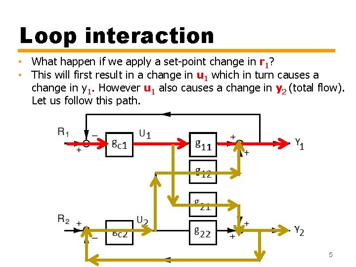
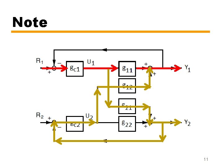
Loop interaction • What happen if we apply a set-point change in r 1? • This will first result in a change in u 1 which in turn causes a change in y 1. However u 1 also causes a change in y 2 (total flow). Let us follow this path. 5

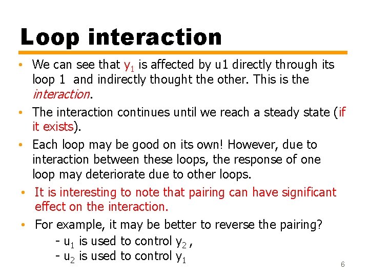
Loop interaction • We can see that y 1 is affected by u 1 directly through its loop 1 and indirectly thought the other. This is the interaction. • The interaction continues until we reach a steady state (if it exists). • Each loop may be good on its own! However, due to interaction between these loops, the response of one loop may deteriorate due to other loops. • It is interesting to note that pairing can have significant effect on the interaction. • For example, it may be better to reverse the pairing? - u 1 is used to control y 2 , - u 2 is used to control y 1 6

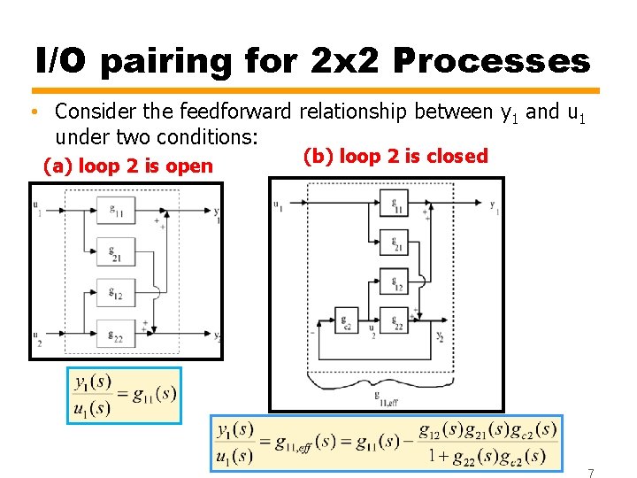
I/O pairing for 2 x 2 Processes • Consider the feedforward relationship between y 1 and u 1 under two conditions: (a) loop 2 is open (b) loop 2 is closed 7

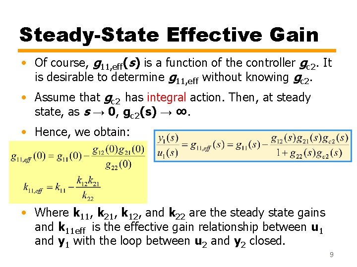
Pairing 2 x 2 Processes • When the second loop (y 2 -u 2) is closed: — there is an additional effect of u 1 on y 1 through the second controller (loop). — This effect can be positive or negative. — g 11, eff(s) is the effective input-output relationship between u 1 and y 1. — This means that g 11, eff(s) should be used as the process transfer function to design controller 1 if loop 2 is closed. 8

Steady-State Effective Gain • Of course, g 11, eff(s) is a function of the controller gc 2. It is desirable to determine g 11, eff without knowing gc 2. • Assume that gc 2 has integral action. Then, at steady state, as s → 0, gc 2(s) → ∞. • Hence, we obtain: • Where k 11, k 21, k 12, and k 22 are the steady state gains and k 11 eff is the effective gain relationship between u 1 and y 1 with the loop between u 2 and y 2 closed. 9

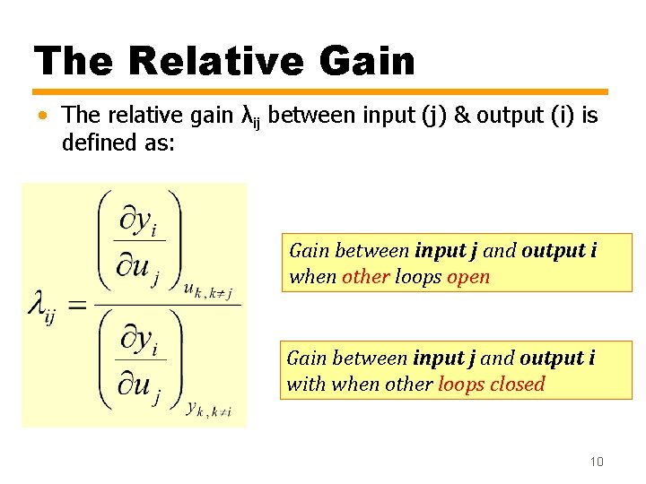
The Relative Gain • The relative gain λij between input (j) & output (i) is defined as: Gain between input j and output i when other loops open Gain between input j and output i with when other loops closed 10

Note 11

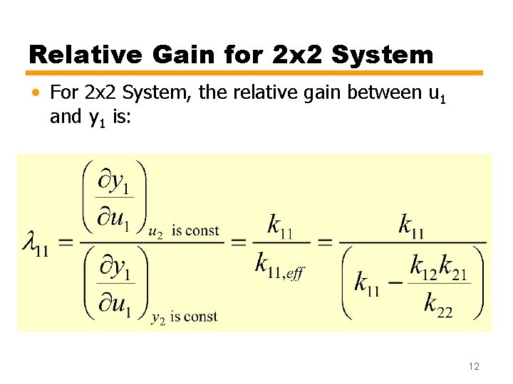
Relative Gain for 2 x 2 System • For 2 x 2 System, the relative gain between u 1 and y 1 is: 12

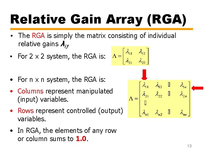
Relative Gain Array (RGA) • The RGA is simply the matrix consisting of individual relative gains λij. • For 2 x 2 system, the RGA is: • For n x n system, the RGA is: • Columns represent manipulated (input) variables. • Rows represent controlled (output) variables. • In RGA, the elements of any row or column sums to 1. 0. 13

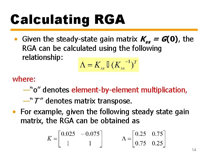
Calculating RGA • Given the steady-state gain matrix Kss = G(0), the RGA can be calculated using the following relationship: where: —“o” denotes element-by-element multiplication, —“T ” denotes matrix transpose. • For example, given the following steady state gain matrix, the RGA can be obtained as 14

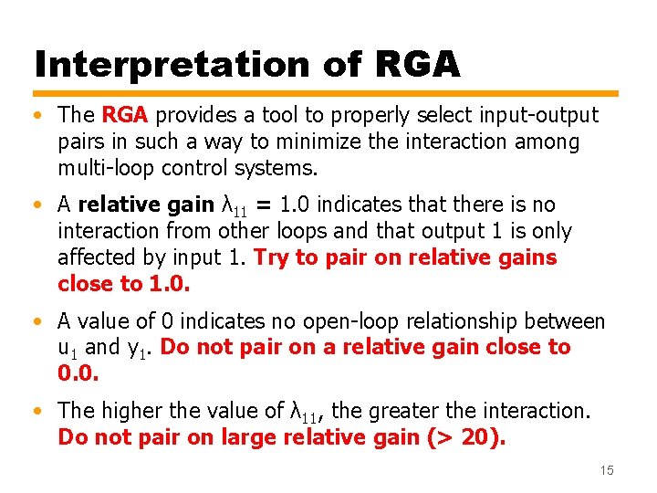
Interpretation of RGA • The RGA provides a tool to properly select input-output pairs in such a way to minimize the interaction among multi-loop control systems. • A relative gain λ 11 = 1. 0 indicates that there is no interaction from other loops and that output 1 is only affected by input 1. Try to pair on relative gains close to 1. 0. • A value of 0 indicates no open-loop relationship between u 1 and y 1. Do not pair on a relative gain close to 0. 0. • The higher the value of λ 11, the greater the interaction. Do not pair on large relative gain (> 20). 15

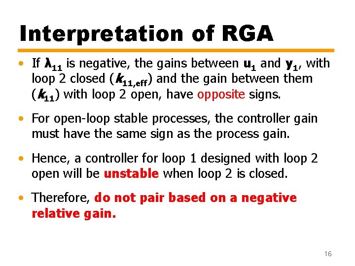
Interpretation of RGA • If λ 11 is negative, the gains between u 1 and y 1, with loop 2 closed (k 11, eff) and the gain between them (k 11) with loop 2 open, have opposite signs. • For open-loop stable processes, the controller gain must have the same sign as the process gain. • Hence, a controller for loop 1 designed with loop 2 open will be unstable when loop 2 is closed. • Therefore, do not pair based on a negative relative gain. 16

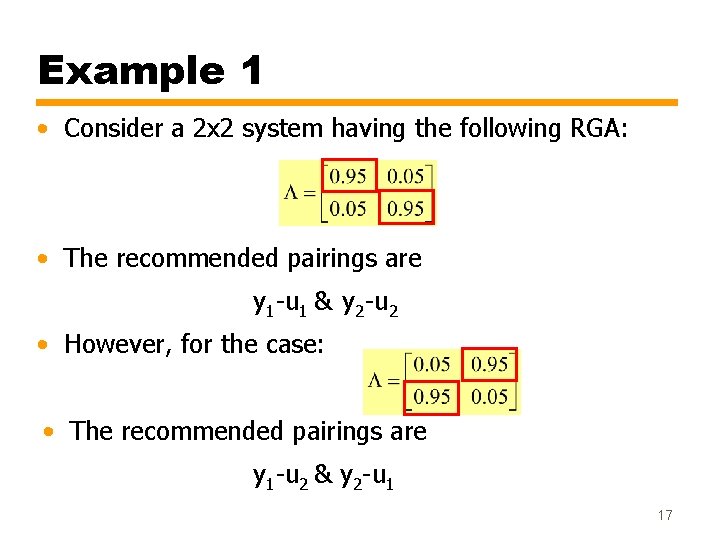
Example 1 • Consider a 2 x 2 system having the following RGA: • The recommended pairings are y 1 -u 1 & y 2 -u 2 • However, for the case: • The recommended pairings are y 1 -u 2 & y 2 -u 1 17

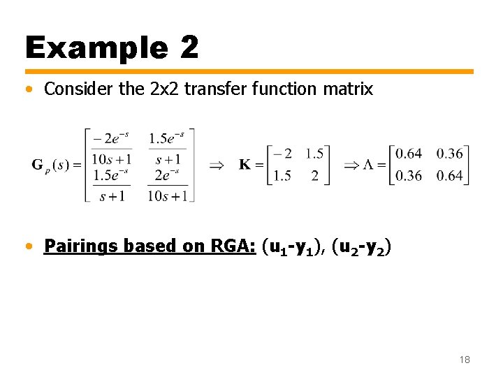
Example 2 • Consider the 2 x 2 transfer function matrix • Pairings based on RGA: (u 1 -y 1), (u 2 -y 2) 18

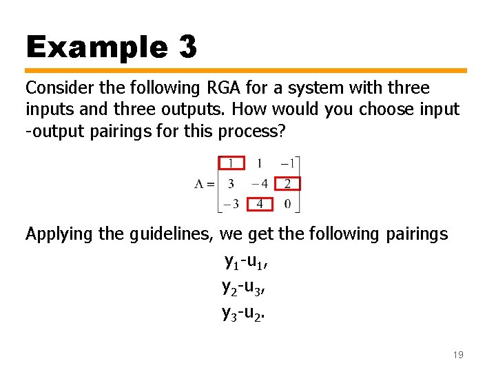
Example 3 Consider the following RGA for a system with three inputs and three outputs. How would you choose input -output pairings for this process? Applying the guidelines, we get the following pairings y 1 -u 1, y 2 -u 3, y 3 -u 2. 19

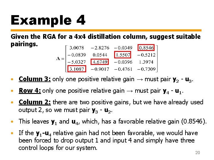
Example 4 Given the RGA for a 4 x 4 distillation column, suggest suitable pairings. • Column 3: only one positive relative gain → must pair y 2 - u 3. • Row 4: only one positive relative gain → must pair y 4 - u 1. • Column 2: there are two positive gains, but we have already used output 2, so we must pair y 3 - u 2. • This leaves y 1 and u 4, which, has a favorable relative gain (0. 8546). • If the y 1 -u 4 relative gain had not been favorable, we would have been forced to drop output 1 and input 4 and simply have three control loops for our system. 20