CONTROL FLOW GRAPHS PROGRAM ANALYSIS AND OPTIMIZATION DCC

CONTROL FLOW GRAPHS PROGRAM ANALYSIS AND OPTIMIZATION – DCC 888 Fernando Magno Quintão Pereira The material in these slides have been taken from the "Dragon Book", Secs 8. 5 – 8. 7, by Aho et al.

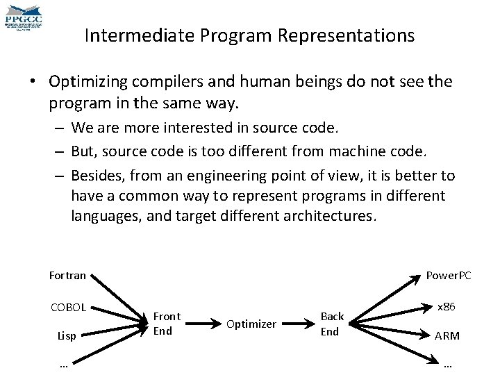
Intermediate Program Representations • Optimizing compilers and human beings do not see the program in the same way. – We are more interested in source code. – But, source code is too different from machine code. – Besides, from an engineering point of view, it is better to have a common way to represent programs in different languages, and target different architectures. Fortran Power. PC COBOL x 86 Lisp … Front End Optimizer Back End ARM …

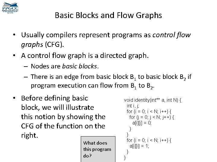
Basic Blocks and Flow Graphs • Usually compilers represent programs as control flow graphs (CFG). • A control flow graph is a directed graph. – Nodes are basic blocks. – There is an edge from basic block B 1 to basic block B 2 if program execution can flow from B 1 to B 2. • Before defining basic block, we will illustrate this notion by showing the CFG of the function on the right. What does this program do? void identity(int** a, int N) { int i, j; for (i = 0; i < N; i++) { for (j = 0; j < N; j++) { a[i][j] = 0; } } for (i = 0; i < N; i++) { a[i][i] = 1; } }

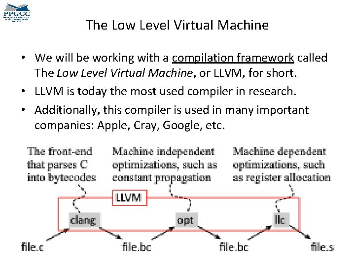
The Low Level Virtual Machine • We will be working with a compilation framework called The Low Level Virtual Machine, or LLVM, for short. • LLVM is today the most used compiler in research. • Additionally, this compiler is used in many important companies: Apple, Cray, Google, etc.

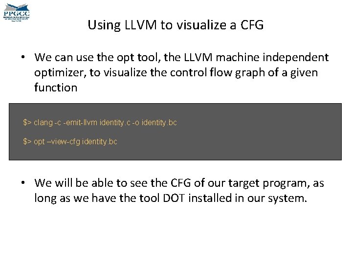
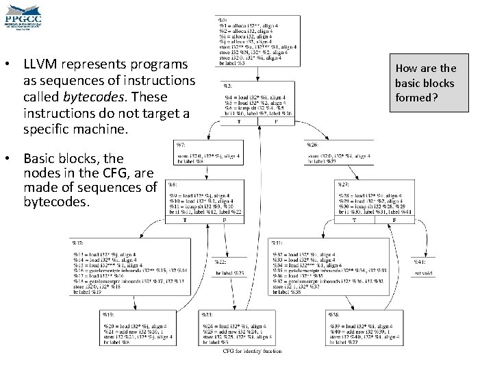
Using LLVM to visualize a CFG • We can use the opt tool, the LLVM machine independent optimizer, to visualize the control flow graph of a given function $> clang -c -emit-llvm identity. c -o identity. bc $> opt –view-cfg identity. bc • We will be able to see the CFG of our target program, as long as we have the tool DOT installed in our system.

The CFG that LLVM produces • LLVM represents programs as sequences of instructions called bytecodes. These instructions do not target a specific machine. • Basic blocks, the nodes in the CFG, are made of sequences of bytecodes. How are the basic blocks formed?

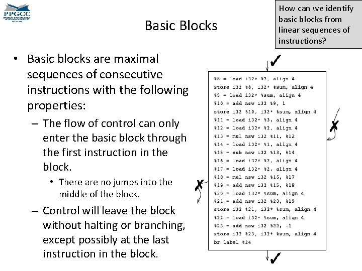
Basic Blocks • Basic blocks are maximal sequences of consecutive instructions with the following properties: – The flow of control can only enter the basic block through the first instruction in the block. • There are no jumps into the middle of the block. – Control will leave the block without halting or branching, except possibly at the last instruction in the block. How can we identify basic blocks from linear sequences of instructions?

Identifying Basic Blocks • The first instruction of a basic block is called a leader. Can you think on a way to identify leaders?

Identifying Basic Blocks • We can identity leaders via these three properties: 1. The first instruction in the intermediate code is a leader. 2. Any instruction that is the target of a conditional or unconditional jump is a leader. 3. Any instruction that immediately follows a conditional or unconditional jump is a leader. Once we have found the leaders, how can we identify the basic blocks?

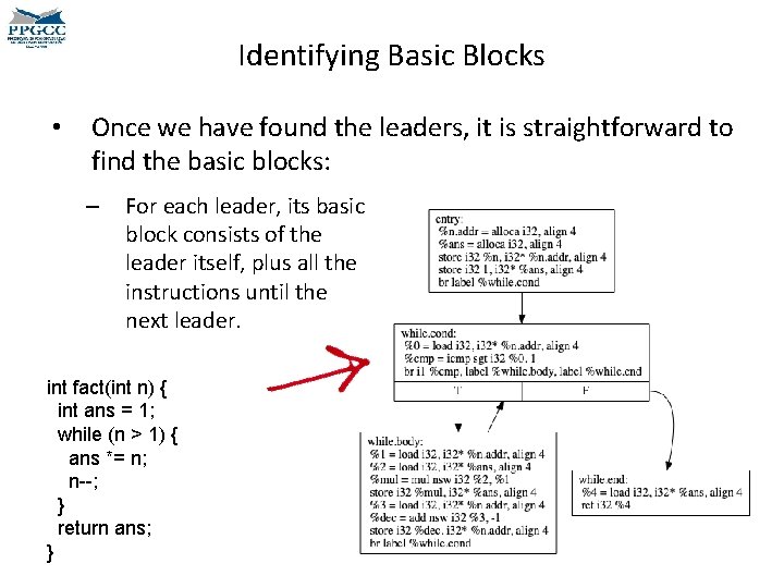
Identifying Basic Blocks • Once we have found the leaders, it is straightforward to find the basic blocks: – For each leader, its basic block consists of the leader itself, plus all the instructions until the next leader. int fact(int n) { int ans = 1; while (n > 1) { ans *= n; n--; } return ans; }

DEPARTMENT OF COMPUTER SCIENCE UNIVERSIDADE FEDERAL DE MINAS GERAIS FEDERAL UNIVERSITY OF MINAS GERAIS, BRAZIL LOCAL OPTIMIZATIONS DCC 888

Local Optimization • Code optimization techniques that work in the scope of a basic block are called local optimizations. – DAG based optimizations – Peephole optimizations – Local register allocation 1) Can you think about a concrete local optimization? • Code optimization techniques that need to analyze the entire control flow graph of a program are called global optimizations. – Most of the optimizations that we will see in this course are global optimizations. 2) Can you think about any global optimization? 3) Can you think about any larger scope of optimization?

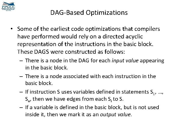
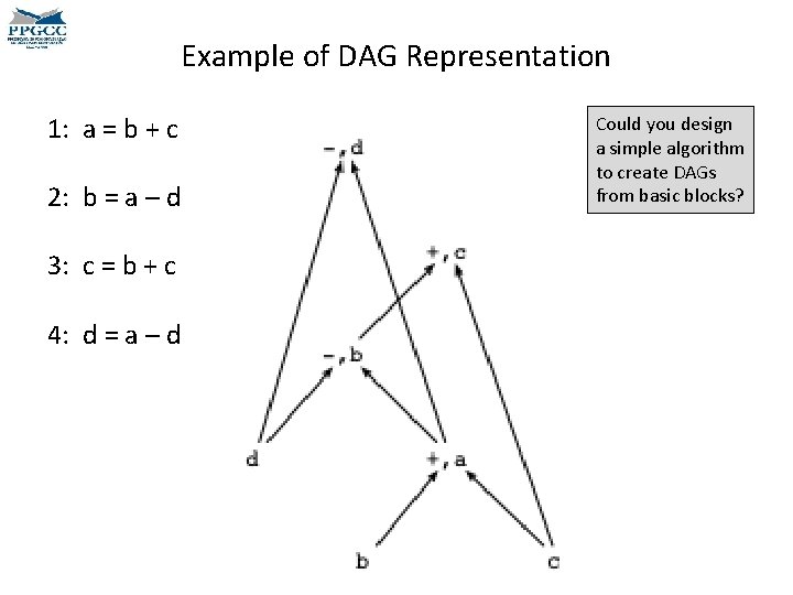
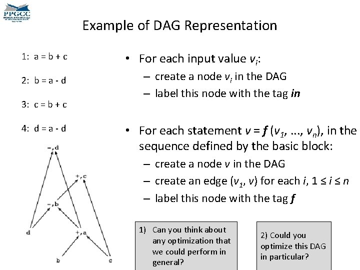
DAG-Based Optimizations • Some of the earliest code optimizations that compilers have performed would rely on a directed acyclic representation of the instructions in the basic block. These DAGS were constructed as follows: – There is a node in the DAG for each input value appearing in the basic block. – There is a node associated with each instruction in the basic block. – If instruction S uses variables defined in statements S 1, …, Sn, then we have edges from each Si to S. – If a variable is defined in the basic block, but is not used inside it, then we mark it as an output value.

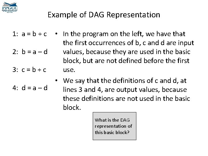
Example of DAG Representation 1: a = b + c • In the program on the left, we have that the first occurrences of b, c and d are input 2: b = a – d values, because they are used in the basic block, but are not defined before the first 3: c = b + c use. • We say that the definitions of c and d, at 4: d = a – d lines 3 and 4, are output values, because these definitions are not used in the basic block. What is the DAG representation of this basic block?

Example of DAG Representation 1: a = b + c 2: b = a – d 3: c = b + c 4: d = a – d Could you design a simple algorithm to create DAGs from basic blocks?

Example of DAG Representation 1: a = b + c 2: b = a - d 3: c = b + c 4: d = a - d • For each input value vi: – create a node vi in the DAG – label this node with the tag in • For each statement v = f (v 1, . . . , vn), in the sequence defined by the basic block: – create a node v in the DAG – create an edge (v 1, v) for each i, 1 ≤ i ≤ n – label this node with the tag f 1) Can you think about any optimization that we could perform in general? 2) Could you optimize this DAG in particular?

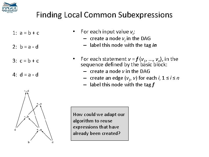
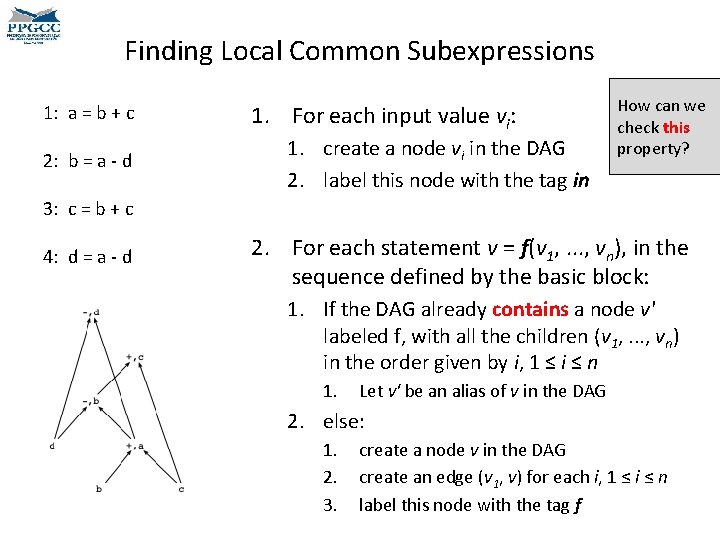
Finding Local Common Subexpressions 1: a = b + c 2: b = a - d 3: c = b + c 4: d = a - d • For each input value vi: – create a node vi in the DAG – label this node with the tag in • For each statement v = f (v 1, . . . , vn), in the sequence defined by the basic block: – create a node v in the DAG – create an edge (v 1, v) for each i, 1 ≤ i ≤ n – label this node with the tag f How could we adapt our algorithm to reuse expressions that have already been created?

Finding Local Common Subexpressions 1: a = b + c 2: b = a - d 1. For each input value vi: 1. create a node vi in the DAG 2. label this node with the tag in How can we check this property? 3: c = b + c 4: d = a - d 2. For each statement v = f(v 1, . . . , vn), in the sequence defined by the basic block: 1. If the DAG already contains a node v' labeled f, with all the children (v 1, . . . , vn) in the order given by i, 1 ≤ i ≤ n 1. Let v' be an alias of v in the DAG 2. else: 1. 2. 3. create a node v in the DAG create an edge (v 1, v) for each i, 1 ≤ i ≤ n label this node with the tag f

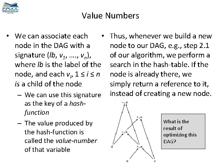
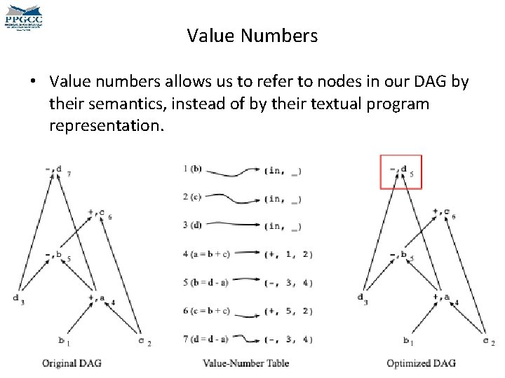
Value Numbers • • We can associate each node in the DAG with a signature (lb, v 1, …. , vn), where lb is the label of the node, and each vi, 1 ≤ i ≤ n is a child of the node – We can use this signature as the key of a hashfunction – The value produced by the hash-function is called the value-number of that variable Thus, whenever we build a new node to our DAG, e. g. , step 2. 1 of our algorithm, we perform a search in the hash-table. If the node is already there, we simply return a reference to it, instead of creating a new node. What is the result of optimizing this DAG?

Value Numbers • Value numbers allows us to refer to nodes in our DAG by their semantics, instead of by their textual program representation.

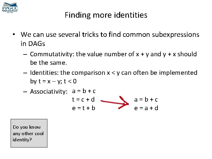
Finding more identities • We can use several tricks to find common subexpressions in DAGs – Commutativity: the value number of x + y and y + x should be the same. – Identities: the comparison x < y can often be implemented by t = x – y; t < 0 – Associativity: a = b + c t=c+d a=b+c e=t+b e=a+d Do you know any other cool identity?

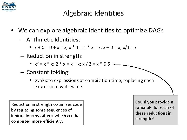
Algebraic Identities • We can explore algebraic identities to optimize DAGs – Arithmetic Identities: • x + 0 = 0 + x = x; x * 1 = 1 * x = x; x – 0 = x; x/1 = x – Reduction in strength: • x 2 = x * x; 2 * x = x + x; x / 2 = x * 0. 5 – Constant folding: • evaluate expressions at compilation time, replacing each expression by its value Reduction in strength optimizes code by replacing some sequences of instructions by others, which can be computed more efficiently. Could you provide a rationale for each of these reductions in strength?

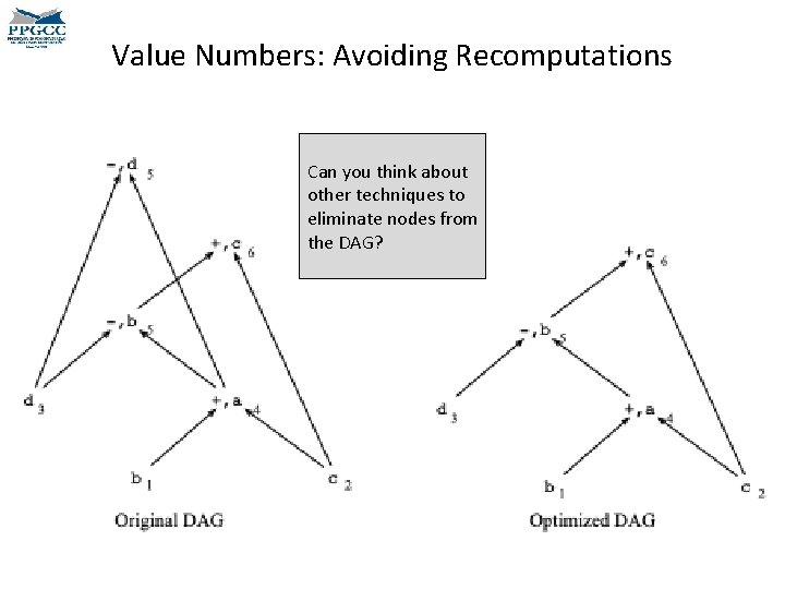
Value Numbers: Avoiding Recomputations Can you think about other techniques to eliminate nodes from the DAG?

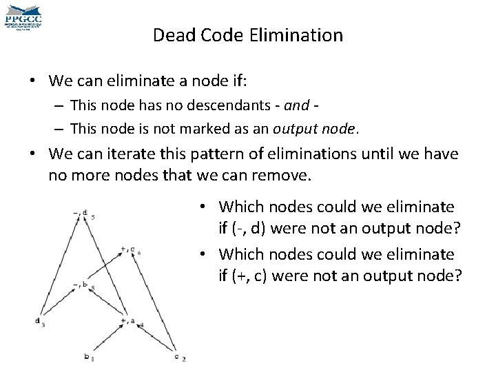
Dead Code Elimination • We can eliminate a node if: – This node has no descendants - and – This node is not marked as an output node. • We can iterate this pattern of eliminations until we have no more nodes that we can remove. • Which nodes could we eliminate if (-, d) were not an output node? • Which nodes could we eliminate if (+, c) were not an output node?

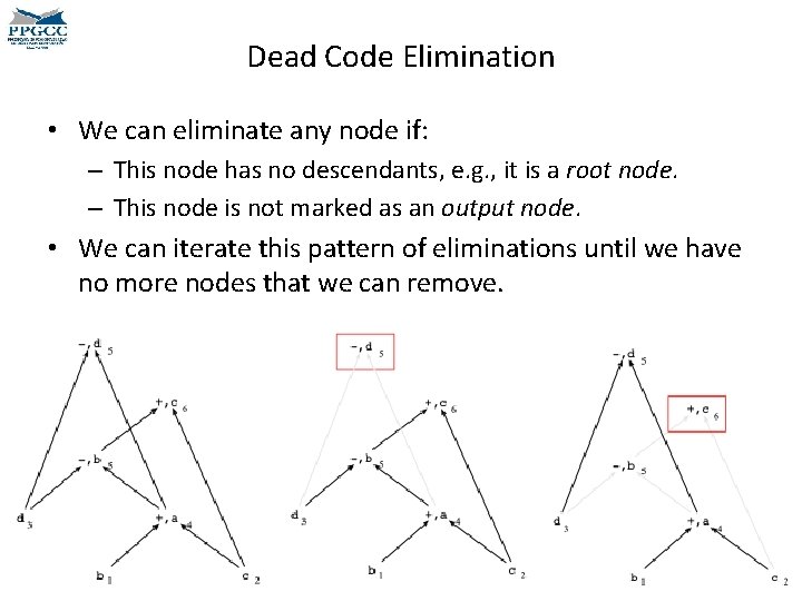
Dead Code Elimination • We can eliminate any node if: – This node has no descendants, e. g. , it is a root node. – This node is not marked as an output node. • We can iterate this pattern of eliminations until we have no more nodes that we can remove.

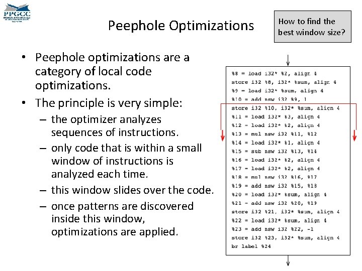
Peephole Optimizations • Peephole optimizations are a category of local code optimizations. • The principle is very simple: – the optimizer analyzes sequences of instructions. – only code that is within a small window of instructions is analyzed each time. – this window slides over the code. – once patterns are discovered inside this window, optimizations are applied. How to find the best window size?

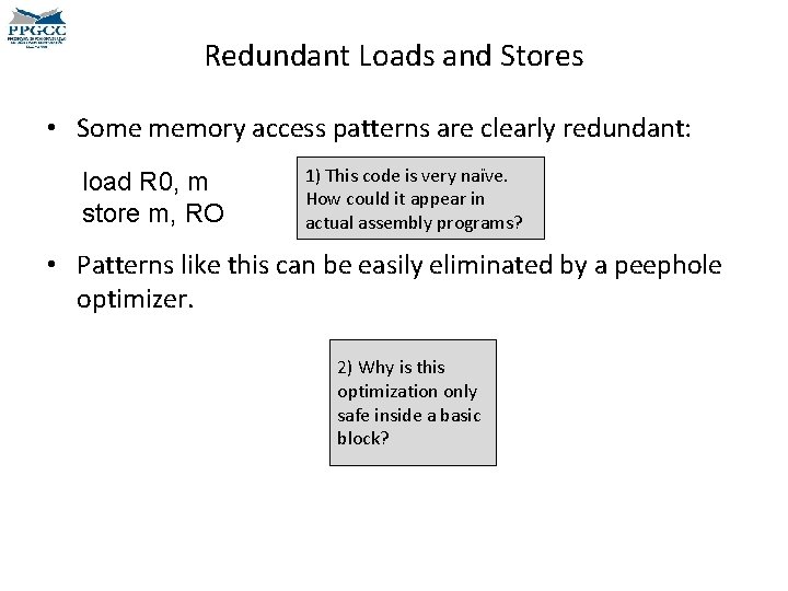
Redundant Loads and Stores • Some memory access patterns are clearly redundant: load R 0, m store m, RO 1) This code is very naïve. How could it appear in actual assembly programs? • Patterns like this can be easily eliminated by a peephole optimizer. 2) Why is this optimization only safe inside a basic block?

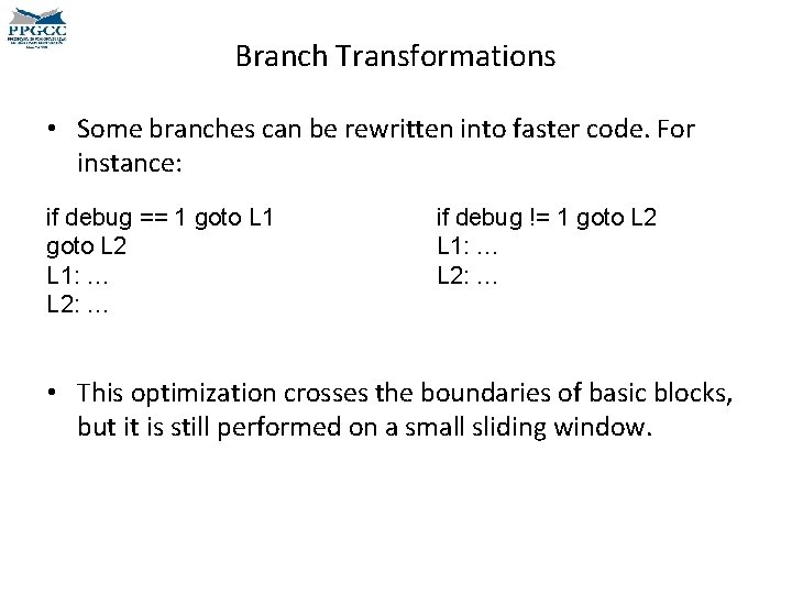
Branch Transformations • Some branches can be rewritten into faster code. For instance: if debug == 1 goto L 2 L 1: … L 2: … if debug != 1 goto L 2 L 1: … L 2: … • This optimization crosses the boundaries of basic blocks, but it is still performed on a small sliding window.

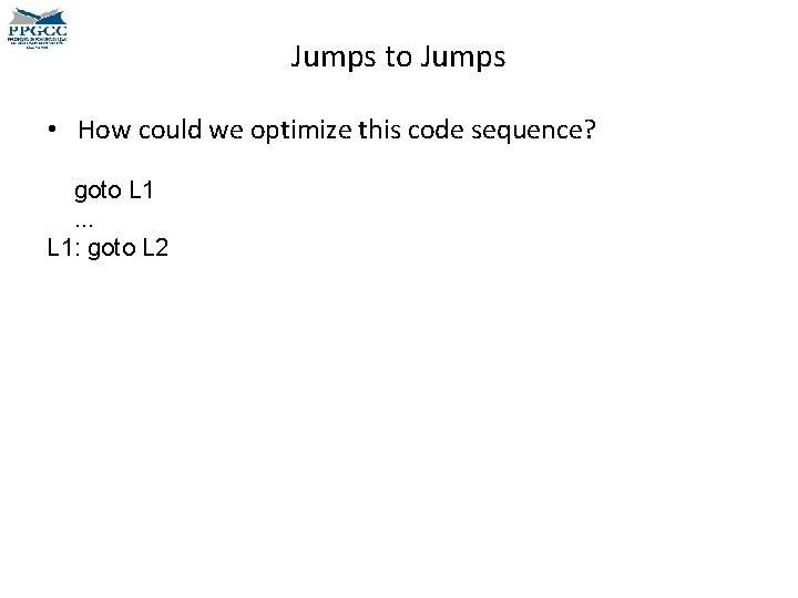
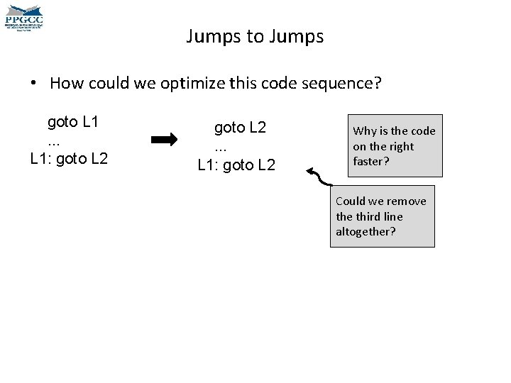
Jumps to Jumps • How could we optimize this code sequence? goto L 1. . . L 1: goto L 2

Jumps to Jumps • How could we optimize this code sequence? goto L 1. . . L 1: goto L 2 Why is the code on the right faster? Could we remove third line altogether?

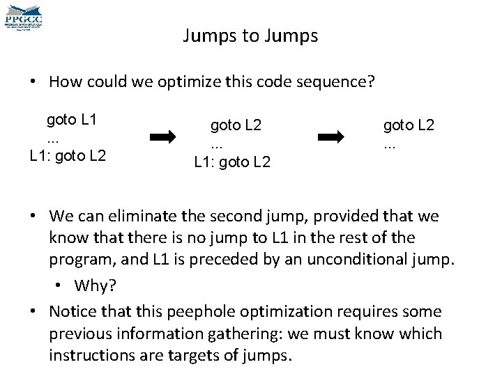
Jumps to Jumps • How could we optimize this code sequence? goto L 1. . . L 1: goto L 2. . . • We can eliminate the second jump, provided that we know that there is no jump to L 1 in the rest of the program, and L 1 is preceded by an unconditional jump. • Why? • Notice that this peephole optimization requires some previous information gathering: we must know which instructions are targets of jumps.

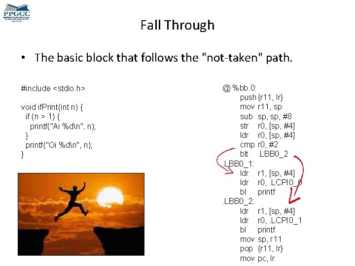
Fall Through • The basic block that follows the "not-taken" path. #include <stdio. h> void if. Print(int n) { if (n > 1) { printf("Ai %dn", n); } printf("Oi %dn", n); } @ %bb. 0: push{r 11, lr} mov r 11, sp sub sp, #8 str r 0, [sp, #4] ldr r 0, [sp, #4] cmp r 0, #2 blt. LBB 0_2. LBB 0_1: ldr r 1, [sp, #4] ldr r 0, . LCPI 0_0 bl printf. LBB 0_2: ldr r 1, [sp, #4] ldr r 0, . LCPI 0_1 bl printf mov sp, r 11 pop {r 11, lr} mov pc, lr

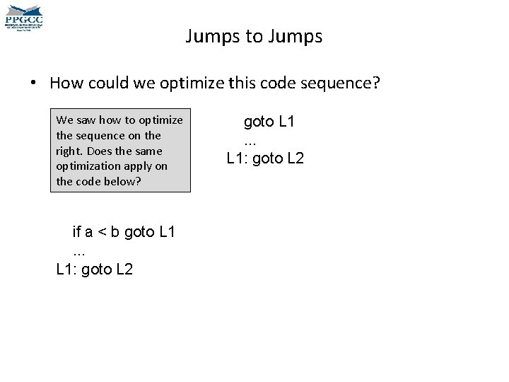
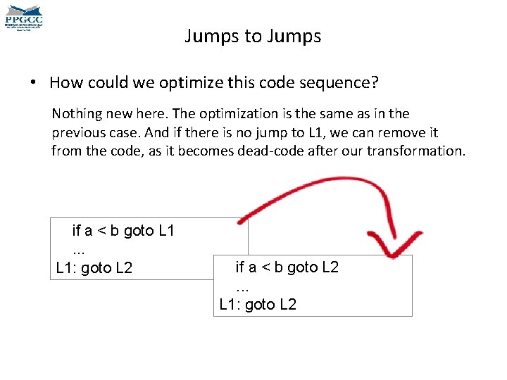
Jumps to Jumps • How could we optimize this code sequence? We saw how to optimize the sequence on the right. Does the same optimization apply on the code below? if a < b goto L 1. . . L 1: goto L 2

Jumps to Jumps • How could we optimize this code sequence? Nothing new here. The optimization is the same as in the previous case. And if there is no jump to L 1, we can remove it from the code, as it becomes dead-code after our transformation. if a < b goto L 1. . . L 1: goto L 2 if a < b goto L 2. . . L 1: goto L 2

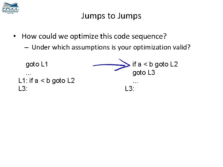
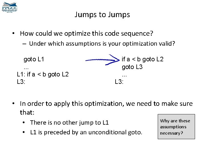
Jumps to Jumps • How could we optimize this code sequence? – Under which assumptions is your optimization valid? goto L 1. . . L 1: if a < b goto L 2 L 3: if a < b goto L 2 goto L 3. . . L 3:

Jumps to Jumps • How could we optimize this code sequence? – Under which assumptions is your optimization valid? goto L 1. . . L 1: if a < b goto L 2 L 3: if a < b goto L 2 goto L 3. . . L 3: • In order to apply this optimization, we need to make sure that: • There is no other jump to L 1 • L 1 is preceded by an unconditional goto. Why are these assumptions necessary?

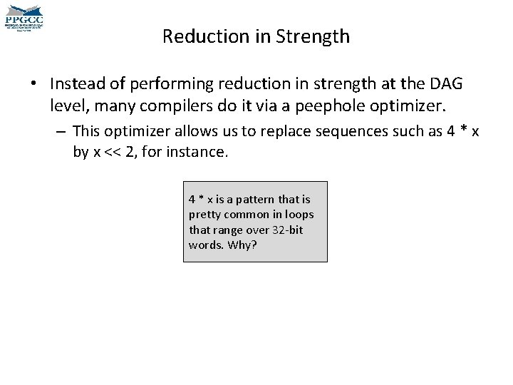
Reduction in Strength • Instead of performing reduction in strength at the DAG level, many compilers do it via a peephole optimizer. – This optimizer allows us to replace sequences such as 4 * x by x << 2, for instance. 4 * x is a pattern that is pretty common in loops that range over 32 -bit words. Why?

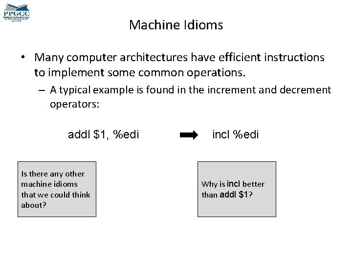
Machine Idioms • Many computer architectures have efficient instructions to implement some common operations. – A typical example is found in the increment and decrement operators: addl $1, %edi Is there any other machine idioms that we could think about? incl %edi Why is incl better than addl $1?

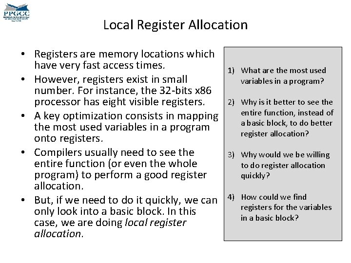
Local Register Allocation • Registers are memory locations which have very fast access times. • However, registers exist in small number. For instance, the 32 -bits x 86 processor has eight visible registers. • A key optimization consists in mapping the most used variables in a program onto registers. • Compilers usually need to see the entire function (or even the whole program) to perform a good register allocation. • But, if we need to do it quickly, we can only look into a basic block. In this case, we are doing local register allocation. 1) What are the most used variables in a program? 2) Why is it better to see the entire function, instead of a basic block, to do better register allocation? 3) Why would we be willing to do register allocation quickly? 4) How could we find registers for the variables in a basic block?

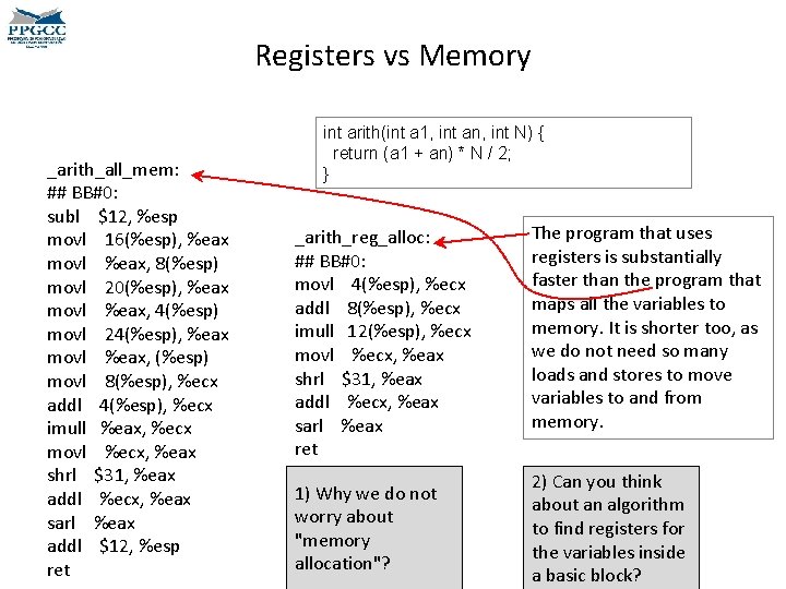
Registers vs Memory _arith_all_mem: ## BB#0: subl $12, %esp movl 16(%esp), %eax movl %eax, 8(%esp) movl 20(%esp), %eax movl %eax, 4(%esp) movl 24(%esp), %eax movl %eax, (%esp) movl 8(%esp), %ecx addl 4(%esp), %ecx imull %eax, %ecx movl %ecx, %eax shrl $31, %eax addl %ecx, %eax sarl %eax addl $12, %esp ret int arith(int a 1, int an, int N) { return (a 1 + an) * N / 2; } _arith_reg_alloc: ## BB#0: movl 4(%esp), %ecx addl 8(%esp), %ecx imull 12(%esp), %ecx movl %ecx, %eax shrl $31, %eax addl %ecx, %eax sarl %eax ret 1) Why we do not worry about "memory allocation"? The program that uses registers is substantially faster than the program that maps all the variables to memory. It is shorter too, as we do not need so many loads and stores to move variables to and from memory. 2) Can you think about an algorithm to find registers for the variables inside a basic block?

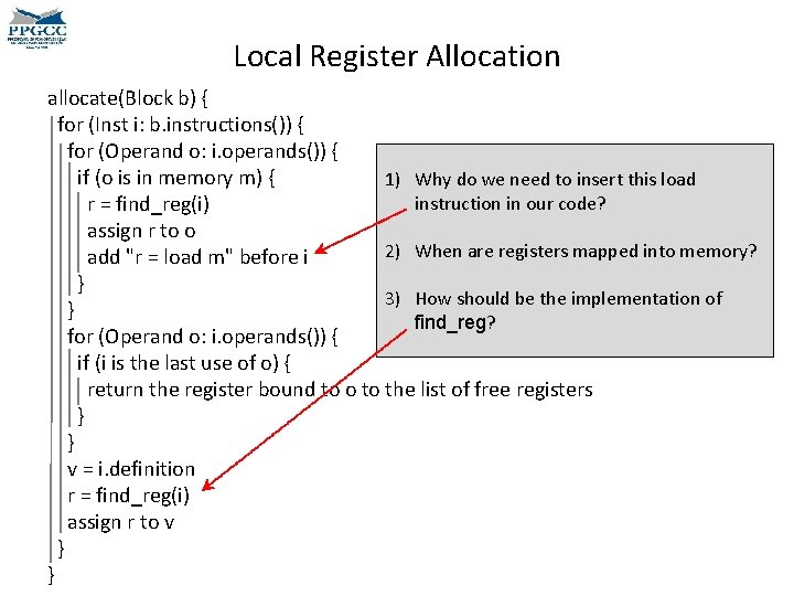
Local Register Allocation allocate(Block b) { for (Inst i: b. instructions()) { for (Operand o: i. operands()) { if (o is in memory m) { 1) Why do we need to insert this load instruction in our code? r = find_reg(i) assign r to o 2) When are registers mapped into memory? add "r = load m" before i } 3) How should be the implementation of } find_reg? for (Operand o: i. operands()) { if (i is the last use of o) { return the register bound to o to the list of free registers } } v = i. definition r = find_reg(i) assign r to v } }

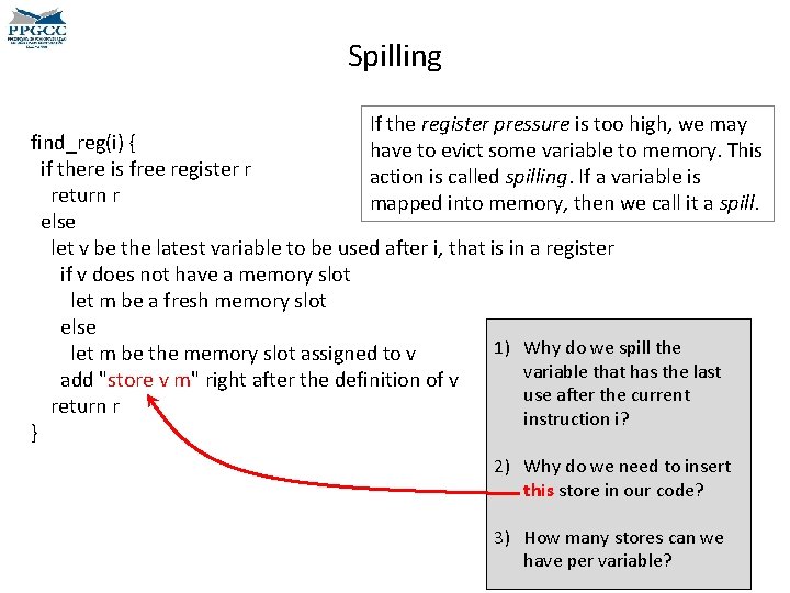
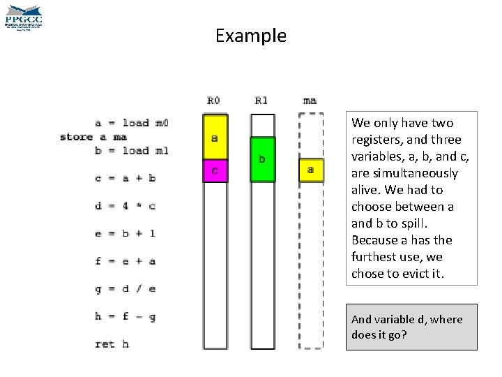
Spilling If the register pressure is too high, we may have to evict some variable to memory. This action is called spilling. If a variable is mapped into memory, then we call it a spill. find_reg(i) { if there is free register r return r else let v be the latest variable to be used after i, that is in a register if v does not have a memory slot let m be a fresh memory slot else 1) Why do we spill the let m be the memory slot assigned to v variable that has the last add "store v m" right after the definition of v use after the current return r instruction i? } 2) Why do we need to insert this store in our code? 3) How many stores can we have per variable?

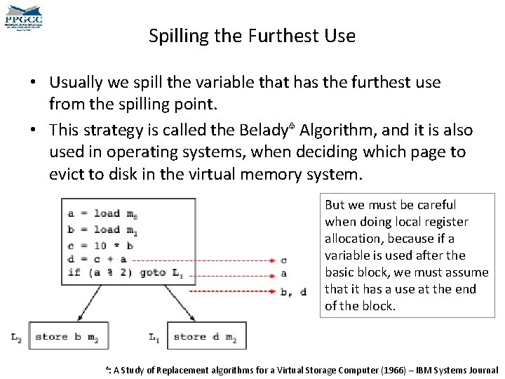
Spilling the Furthest Use • Usually we spill the variable that has the furthest use from the spilling point. • This strategy is called the Belady♧ Algorithm, and it is also used in operating systems, when deciding which page to evict to disk in the virtual memory system. But we must be careful when doing local register allocation, because if a variable is used after the basic block, we must assume that it has a use at the end of the block. ♧: A Study of Replacement algorithms for a Virtual Storage Computer (1966) – IBM Systems Journal

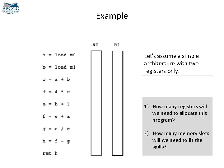
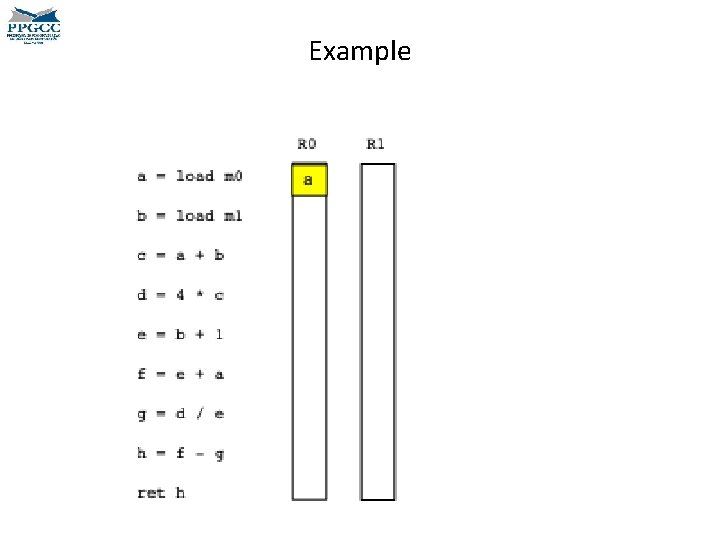
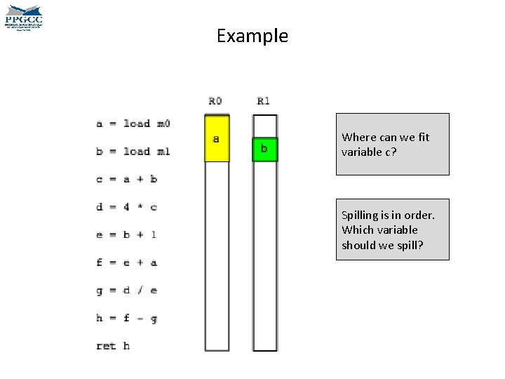
Example Let's assume a simple architecture with two registers only. 1) How many registers will we need to allocate this program? 2) How many memory slots will we need to fit the spills?

Example

Example Where can we fit variable c? Spilling is in order. Which variable should we spill?

Example We only have two registers, and three variables, a, b, and c, are simultaneously alive. We had to choose between a and b to spill. Because a has the furthest use, we chose to evict it. And variable d, where does it go?

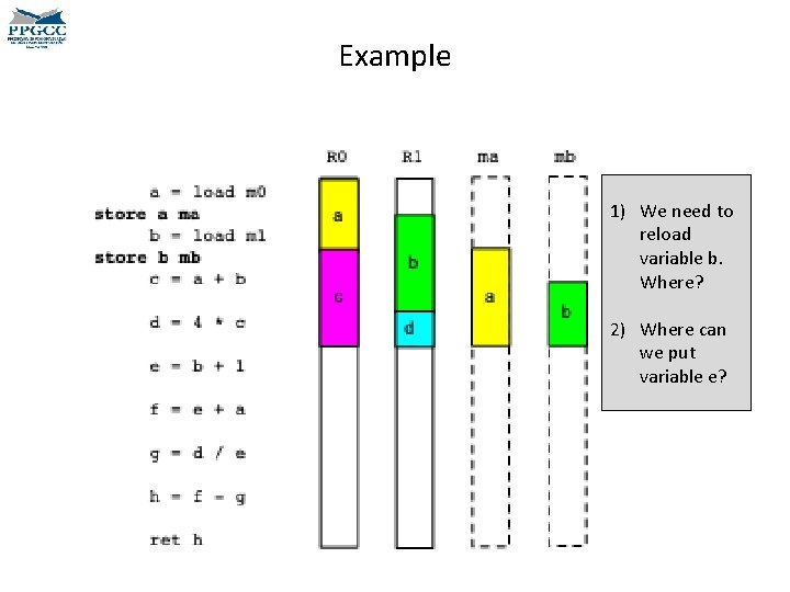
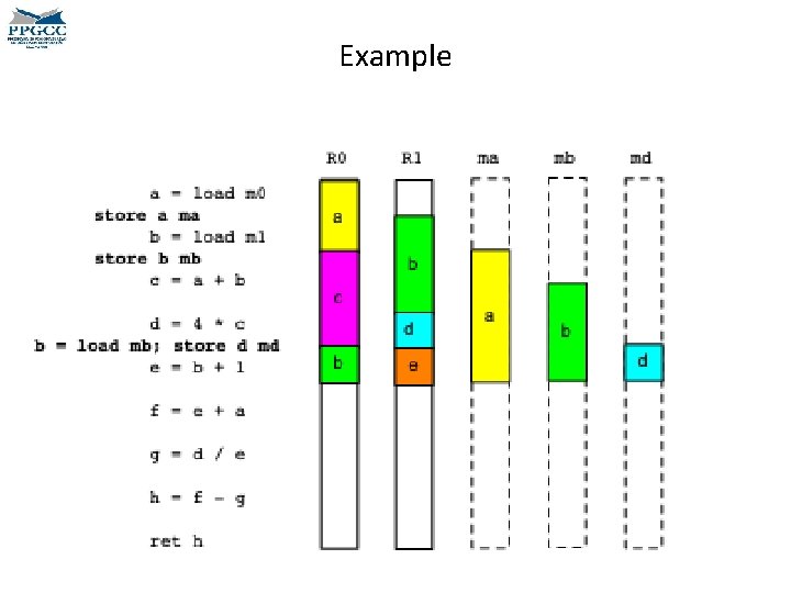
Example 1) We need to reload variable b. Where? 2) Where can we put variable e?

Example

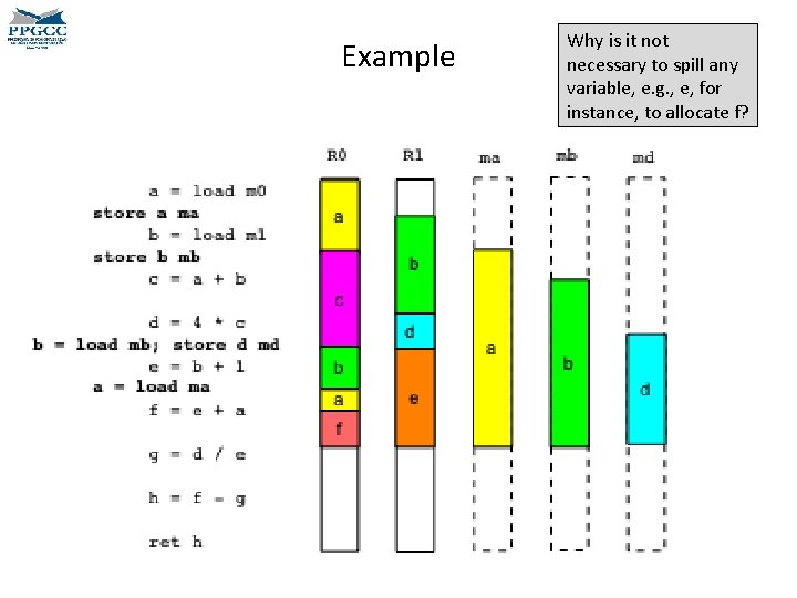
Example Why is it not necessary to spill any variable, e. g. , e, for instance, to allocate f?

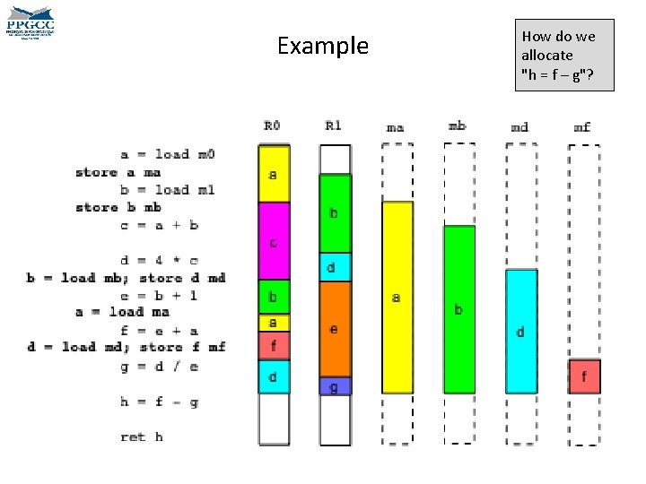
Example How do we allocate "h = f – g"?

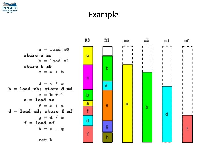
Example

Optimality • If there exists an assignment of variables to registers that requires at most K registers, then our algorithm will find it. – If registers had different sizes, e. g. , singles and doubles, then this problem would be NP-complete¥. • On the other hand, if we need to spill, then the problem of minimizing the cost of loads and stores is NPcomplete♤. ¥: 1) Can you prove that the algorithm is optimal for register assignment? 2) Any intuition on why minimizing this cost is an NPcomplete problem? Aliased register allocation for straight-line programs is NP-complete. Theor. Comp. Sci. , 2008 ♤: On local register allocation, SODA, 1998

DEPARTMENT OF COMPUTER SCIENCE UNIVERSIDADE FEDERAL DE MINAS GERAIS FEDERAL UNIVERSITY OF MINAS GERAIS, BRAZIL A QUICK INTRO TO LLVM DCC 888

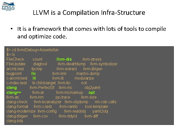
LLVM is a Compilation Infra-Structure • It is a framework that comes with lots of tools to compile and optimize code. $> cd llvm/Debug+Asserts/bin $> ls File. Check count llvm-dis llvm-stress File. Update diagtool llvm-dwarfdump llvm-symbolizer arcmt-test fpcmp llvm-extract llvm-tblgen bugpoint llc llvm-link macho-dump c-arcmt-test lli llvm-lit modularize c-index-test lli-child-target llvm-lto not clang llvm-Perfect. Sf llvm-mc obj 2 yaml clang++ llvm-ar llvm-mcmarkup opt llvm-as llvm-nm pp-trace llvm-size clang-check llvm-bcanalyzer llvm-objdump rm-cstr-calls clang-format llvm-c-test llvm-ranlib tool-template clang-modernize llvm-config llvm-readobj yaml 2 obj clang-tblgen llvm-cov llvm-rtdyld llvm-diff clang-tidy

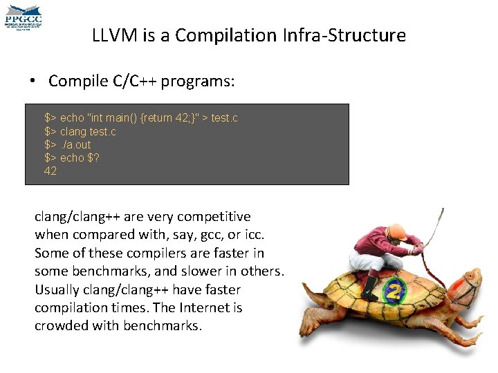
LLVM is a Compilation Infra-Structure • Compile C/C++ programs: $> echo "int main() {return 42; }" > test. c $> clang test. c $>. /a. out $> echo $? 42 clang/clang++ are very competitive when compared with, say, gcc, or icc. Some of these compilers are faster in some benchmarks, and slower in others. Usually clang/clang++ have faster compilation times. The Internet is crowded with benchmarks.

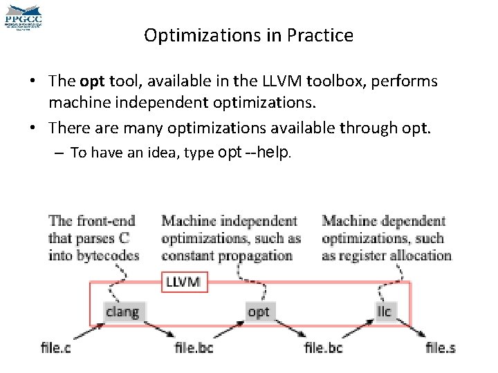
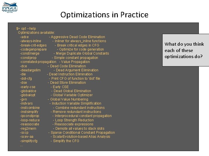
Optimizations in Practice • The opt tool, available in the LLVM toolbox, performs machine independent optimizations. • There are many optimizations available through opt. – To have an idea, type opt --help.

Optimizations in Practice $> opt --help Optimizations available: -adce - Aggressive Dead Code Elimination -always-inline - Inliner for always_inline functions -break-crit-edges - Break critical edges in CFG -codegenprepare - Optimize for code generation -constmerge - Merge Duplicate Global Constants -constprop - Simple constant propagation -correlated-propagation - Value Propagation -dce - Dead Code Elimination -deadargelim - Dead Argument Elimination -die - Dead Instruction Elimination -dot-cfg - Print CFG of function to 'dot' file -dse - Dead Store Elimination -early-cse - Early CSE -globaldce - Dead Global Elimination -globalopt - Global Variable Optimizer -gvn - Global Value Numbering -indvars - Induction Variable Simplification -instcombine - Combine redundant instructions -instsimplify - Remove redundant instructions -ipconstprop - Interprocedural constant propagation -loop-reduce - Loop Strength Reduction -reassociate - Reassociate expressions -reg 2 mem - Demote all values to stack slots -sccp - Sparse Conditional Constant Propagation -scev-aa - Scalar. Evolution-based Alias Analysis -simplifycfg - Simplify the CFG. . . What do you think each of these optimizations do?

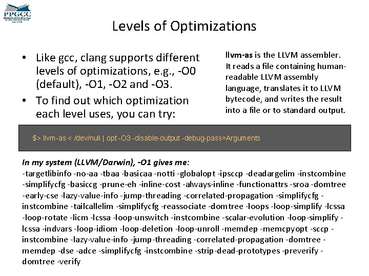
Levels of Optimizations • Like gcc, clang supports different levels of optimizations, e. g. , -O 0 (default), -O 1, -O 2 and -O 3. • To find out which optimization each level uses, you can try: llvm-as is the LLVM assembler. It reads a file containing humanreadable LLVM assembly language, translates it to LLVM bytecode, and writes the result into a file or to standard output. $> llvm-as < /dev/null | opt -O 3 -disable-output -debug-pass=Arguments In my system (LLVM/Darwin), -O 1 gives me: -targetlibinfo -no-aa -tbaa -basicaa -notti -globalopt -ipsccp -deadargelim -instcombine -simplifycfg -basiccg -prune-eh -inline-cost -always-inline -functionattrs -sroa -domtree -early-cse -lazy-value-info -jump-threading -correlated-propagation -simplifycfg instcombine -tailcallelim -simplifycfg -reassociate -domtree -loops -loop-simplify -lcssa -loop-rotate -licm -lcssa -loop-unswitch -instcombine -scalar-evolution -loop-simplify lcssa -indvars -loop-idiom -loop-deletion -loop-unroll -memdep -memcpyopt -sccp instcombine -lazy-value-info -jump-threading -correlated-propagation -domtree memdep -dse -adce -simplifycfg -instcombine -strip-dead-prototypes -preverify domtree -verify

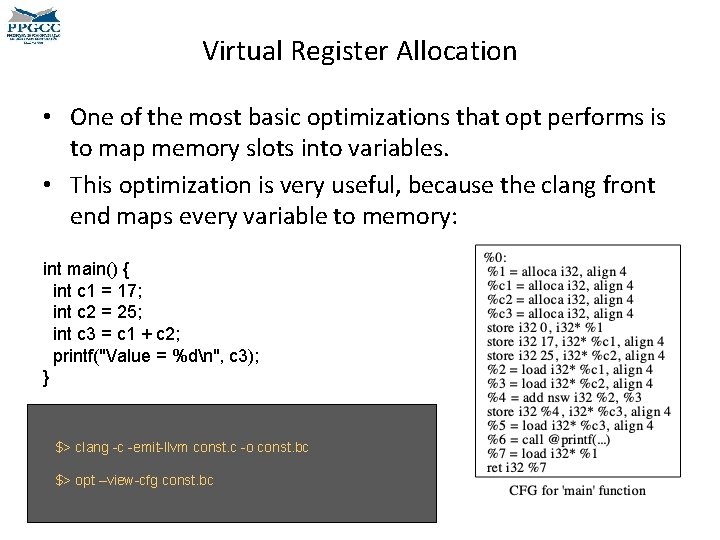
Virtual Register Allocation • One of the most basic optimizations that opt performs is to map memory slots into variables. • This optimization is very useful, because the clang front end maps every variable to memory: int main() { int c 1 = 17; int c 2 = 25; int c 3 = c 1 + c 2; printf("Value = %dn", c 3); } $> clang -c -emit-llvm const. c -o const. bc $> opt –view-cfg const. bc

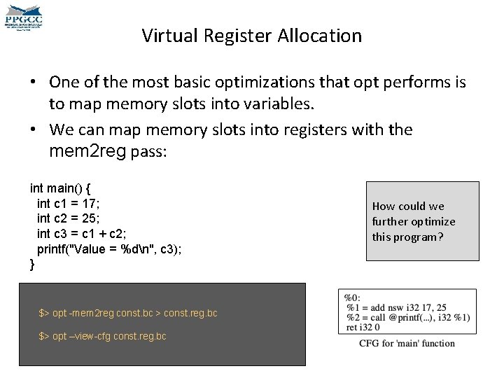
Virtual Register Allocation • One of the most basic optimizations that opt performs is to map memory slots into variables. • We can map memory slots into registers with the mem 2 reg pass: int main() { int c 1 = 17; int c 2 = 25; int c 3 = c 1 + c 2; printf("Value = %dn", c 3); } $> opt -mem 2 reg const. bc > const. reg. bc $> opt –view-cfg const. reg. bc How could we further optimize this program?

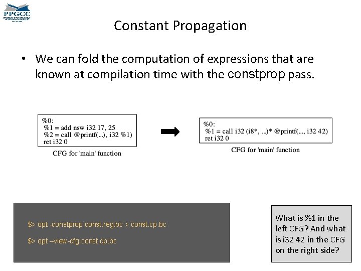
Constant Propagation • We can fold the computation of expressions that are known at compilation time with the constprop pass. $> opt -constprop const. reg. bc > const. cp. bc $> opt –view-cfg const. cp. bc What is %1 in the left CFG? And what is i 32 42 in the CFG on the right side?

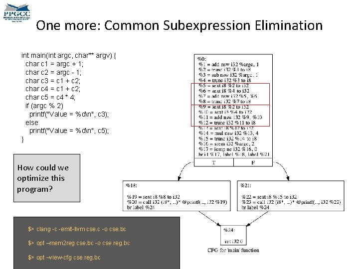
One more: Common Subexpression Elimination int main(int argc, char** argv) { char c 1 = argc + 1; char c 2 = argc - 1; char c 3 = c 1 + c 2; char c 4 = c 1 + c 2; char c 5 = c 4 * 4; if (argc % 2) printf("Value = %dn", c 3); else printf("Value = %dn", c 5); } How could we optimize this program? $> clang -c -emit-llvm cse. c -o cse. bc $> opt –mem 2 reg cse. bc -o cse. reg. bc $> opt –view-cfg cse. reg. bc

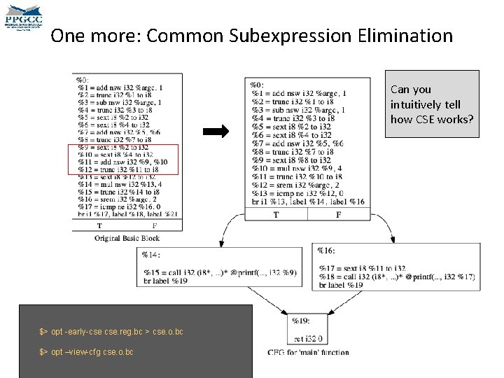
One more: Common Subexpression Elimination Can you intuitively tell how CSE works? $> opt -early-cse cse. reg. bc > cse. o. bc $> opt –view-cfg cse. o. bc

Writing an LLVM pass • LLVM applies a chain of analyses and transformations on the target program. • Each of these analyses or transformations is called a pass. • We have seen a few passes already: mem 2 reg, early-cse and constprop, for instance. • Some passes, which are machine independent, are invoked by the opt tool. • Other passes, which are machine dependent, are invoked by the llc tool. • A pass may require information provided by other passes. Such dependencies must be explicitly stated. – For instance: a common pattern is a transformation pass requiring an analysis pass.

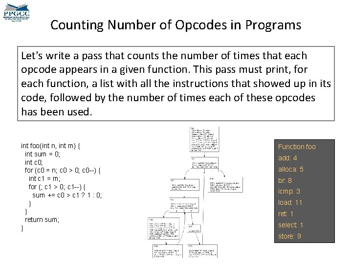
Counting Number of Opcodes in Programs Let's write a pass that counts the number of times that each opcode appears in a given function. This pass must print, for each function, a list with all the instructions that showed up in its code, followed by the number of times each of these opcodes has been used. int foo(int n, int m) { int sum = 0; int c 0; for (c 0 = n; c 0 > 0; c 0 --) { int c 1 = m; for (; c 1 > 0; c 1 --) { sum += c 0 > c 1 ? 1 : 0; } } return sum; } Function foo add: 4 alloca: 5 br: 8 icmp: 3 load: 11 ret: 1 select: 1 store: 9

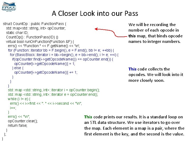
Counting Number of Opcodes in Programs #define DEBUG_TYPE "op. Counter" #include "llvm/Pass. h" #include "llvm/IR/Function. h" #include "llvm/Support/raw_ostream. h" #include <map> using namespace llvm; namespace { struct Count. Op : public Function. Pass { std: : map<std: : string, int> op. Counter; static char ID; Count. Op() : Function. Pass(ID) {} virtual bool run. On. Function(Function &F) { errs() << "Function " << F. get. Name() << 'n'; for (Function: : iterator bb = F. begin(), e = F. end(); bb != e; ++bb) { for (Basic. Block: : iterator i = bb->begin(), e = bb->end(); i != e; ++i) { if(op. Counter. find(i->get. Opcode. Name()) == op. Counter. end()) { op. Counter[i->get. Opcode. Name()] = 1; } else { op. Counter[i->get. Opcode. Name()] += 1; } } } std: : map <std: : string, int>: : iterator i = op. Counter. begin(); std: : map <std: : string, int>: : iterator e = op. Counter. end(); while (i != e) { errs() << i->first << ": " << i->second << "n"; i++; } errs() << "n"; op. Counter. clear(); return false; } }; } char Count. Op: : ID = 0; static Register. Pass<Count. Op> X("op. Counter", "Counts opcodes per functions"); Our pass runs once for each function in the program; therefore, it is a Function. Pass. If we had to see the whole program, then we would implement a Module. Pass. This line defines the name of the pass, in the command line, e. g. , op. Counter, and the help string that opt provides to the user about the pass.

A Closer Look into our Pass struct Count. Op : public Function. Pass { We will be recording the std: : map<std: : string, int> op. Counter; number of each opcode in static char ID; this map, that binds opcode Count. Op() : Function. Pass(ID) {} virtual bool run. On. Function(Function &F) { names to integer numbers. errs() << "Function " << F. get. Name() << 'n'; for (Function: : iterator bb = F. begin(), e = F. end(); bb != e; ++bb) { for (Basic. Block: : iterator i = bb->begin(), e = bb->end(); i != e; ++i) { if(op. Counter. find(i->get. Opcode. Name()) == op. Counter. end()) { op. Counter[i->get. Opcode. Name()] = 1; } else { This code collects the op. Counter[i->get. Opcode. Name()] += 1; opcodes. We will look into it } more closely soon. } } std: : map <std: : string, int>: : iterator i = op. Counter. begin(); std: : map <std: : string, int>: : iterator e = op. Counter. end(); while (i != e) { errs() << i->first << ": " << i->second << "n"; i++; } errs() << "n"; This code prints our results. It is a standard loop on op. Counter. clear(); an STL data structure. We use iterators to go over return false; the map. Each element in a map is a pair, where the } first element is the key, and the second is the value. }; }

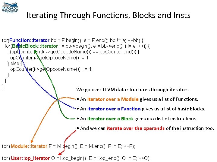
Iterating Through Functions, Blocks and Insts for(Function: : iterator bb = F. begin(), e = F. end(); bb != e; ++bb) { for(Basic. Block: : iterator i = bb->begin(), e = bb->end(); i != e; ++i) { if(op. Counter. find(i->get. Opcode. Name()) == op. Counter. end()) { op. Counter[i->get. Opcode. Name()] = 1; } else { op. Counter[i->get. Opcode. Name()] += 1; } } } We go over LLVM data structures through iterators. • An iterator over a Module gives us a list of Functions. • An iterator over a Function gives us a list of basic blocks. • An iterator over a Block gives us a list of instructions. • And we can iterate over the operands of the instruction too. for (Module: : iterator F = M. begin(), E = M. end(); F != E; ++F); for (User: : op_iterator O = I. op_begin(), E = I. op_end(); O != E; ++O);

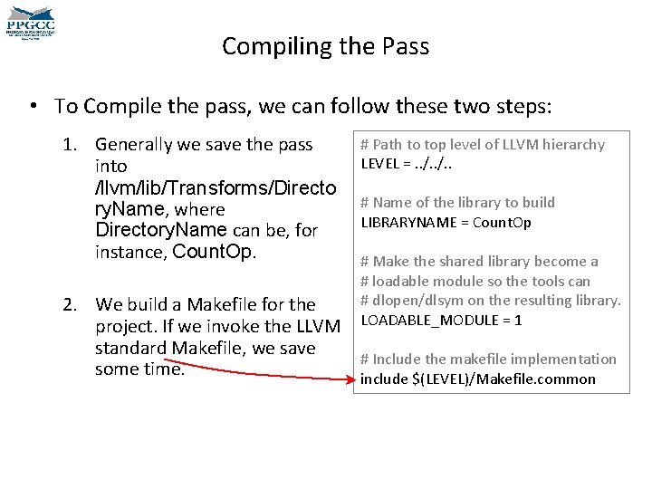
Compiling the Pass • To Compile the pass, we can follow these two steps: 1. Generally we save the pass into /llvm/lib/Transforms/Directo ry. Name, where Directory. Name can be, for instance, Count. Op. 2. We build a Makefile for the project. If we invoke the LLVM standard Makefile, we save some time. # Path to top level of LLVM hierarchy LEVEL =. . /. . # Name of the library to build LIBRARYNAME = Count. Op # Make the shared library become a # loadable module so the tools can # dlopen/dlsym on the resulting library. LOADABLE_MODULE = 1 # Include the makefile implementation include $(LEVEL)/Makefile. common

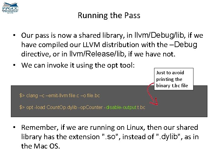
Running the Pass • Our pass is now a shared library, in llvm/Debug/lib, if we have compiled our LLVM distribution with the –Debug directive, or in llvm/Release/lib, if we have not. • We can invoke it using the opt tool: Just to avoid printing the binary t. bc file $> clang –c –emit-llvm file. c –o file. bc $> opt -load Count. Op. dylib -op. Counter -disable-output t. bc • Remember, if we are running on Linux, then our shared library has the extension ". so", instead of ". dylib", as in the Mac OS.

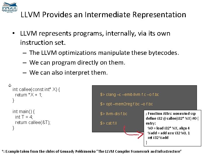
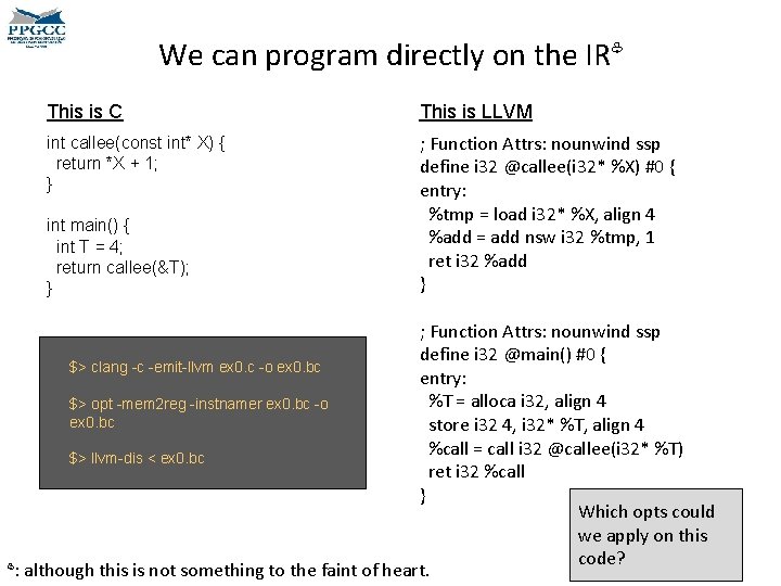
LLVM Provides an Intermediate Representation • LLVM represents programs, internally, via its own instruction set. – The LLVM optimizations manipulate these bytecodes. – We can program directly on them. – We can also interpret them. ♤ int callee(const int* X) { return *X + 1; } int main() { int T = 4; return callee(&T); } ♤: $> clang –c –emit-llvm f. c –o f. bc $> opt –mem 2 reg f. bc –o f. bc $> llvm-dis f. bc $> cat f. ll ; Function Attrs: nounwind ssp define i 32 @callee(i 32* %X) #0 { entry: %0 = load i 32* %X, align 4 %add = add nsw i 32 %0, 1 ret i 32 %add } Example taken from the slides of Gennady Pekhimenko "The LLVM Compiler Framework and Infrastructure"

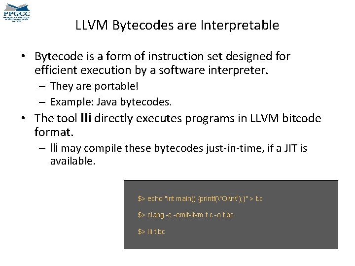
LLVM Bytecodes are Interpretable • Bytecode is a form of instruction set designed for efficient execution by a software interpreter. – They are portable! – Example: Java bytecodes. • The tool lli directly executes programs in LLVM bitcode format. – lli may compile these bytecodes just-in-time, if a JIT is available. $> echo "int main() {printf("Oin"); }" > t. c $> clang -c -emit-llvm t. c -o t. bc $> lli t. bc

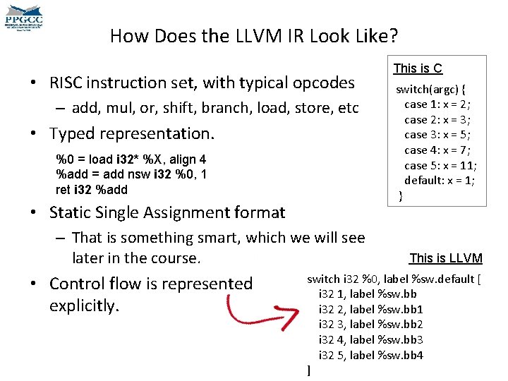
How Does the LLVM IR Look Like? • RISC instruction set, with typical opcodes – add, mul, or, shift, branch, load, store, etc • Typed representation. %0 = load i 32* %X, align 4 %add = add nsw i 32 %0, 1 ret i 32 %add • Static Single Assignment format – That is something smart, which we will see later in the course. • Control flow is represented explicitly. This is C switch(argc) { case 1: x = 2; case 2: x = 3; case 3: x = 5; case 4: x = 7; case 5: x = 11; default: x = 1; } This is LLVM switch i 32 %0, label %sw. default [ i 32 1, label %sw. bb i 32 2, label %sw. bb 1 i 32 3, label %sw. bb 2 i 32 4, label %sw. bb 3 i 32 5, label %sw. bb 4 ]

We can program directly on the IR♧ This is C This is LLVM int callee(const int* X) { return *X + 1; } ; Function Attrs: nounwind ssp define i 32 @callee(i 32* %X) #0 { entry: %tmp = load i 32* %X, align 4 %add = add nsw i 32 %tmp, 1 ret i 32 %add } int main() { int T = 4; return callee(&T); } ; Function Attrs: nounwind ssp define i 32 @main() #0 { $> clang -c -emit-llvm ex 0. c -o ex 0. bc entry: %T = alloca i 32, align 4 $> opt -mem 2 reg -instnamer ex 0. bc -o ex 0. bc store i 32 4, i 32* %T, align 4 %call = call i 32 @callee(i 32* %T) $> llvm-dis < ex 0. bc ret i 32 %call } Which opts could we apply on this code? ♧: although this is not something to the faint of heart.

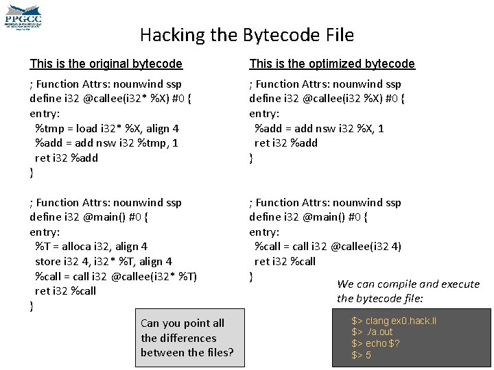
Hacking the Bytecode File This is the original bytecode This is the optimized bytecode ; Function Attrs: nounwind ssp define i 32 @callee(i 32* %X) #0 { entry: %tmp = load i 32* %X, align 4 %add = add nsw i 32 %tmp, 1 ret i 32 %add } ; Function Attrs: nounwind ssp define i 32 @callee(i 32 %X) #0 { entry: %add = add nsw i 32 %X, 1 ret i 32 %add } ; Function Attrs: nounwind ssp define i 32 @main() #0 { entry: %T = alloca i 32, align 4 store i 32 4, i 32* %T, align 4 %call = call i 32 @callee(i 32* %T) ret i 32 %call } Can you point all the differences between the files? ; Function Attrs: nounwind ssp define i 32 @main() #0 { entry: %call = call i 32 @callee(i 32 4) ret i 32 %call } We can compile and execute the bytecode file: $> clang ex 0. hack. ll $>. /a. out $> echo $? $> 5

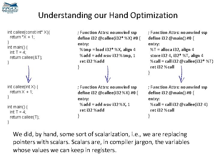
Understanding our Hand Optimization int callee(const int* X){ return *X + 1; } int main() { int T = 4; return callee(&T); } ; Function Attrs: nounwind ssp define i 32 @callee(i 32* %X) #0 { entry: %tmp = load i 32* %X, align 4 %add = add nsw i 32 %tmp, 1 ret i 32 %add } ; Function Attrs: nounwind ssp define i 32 @main() #0 { entry: %T = alloca i 32, align 4 store i 32 4, i 32* %T, align 4 %call = call i 32 @callee(i 32* %T) ret i 32 %call } int callee(int X) { return X + 1; } ; Function Attrs: nounwind ssp define i 32 @callee(i 32 %X) #0 { entry: %add = add nsw i 32 %X, 1 ret i 32 %add } ; Function Attrs: nounwind ssp define i 32 @main() #0 { entry: %call = call i 32 @callee(i 32 4) ret i 32 %call } int main() { int T = 4; return callee(T); } We did, by hand, some sort of scalarization, i. e. , we are replacing pointers with scalars. Scalars are, in compiler jargon, the variables whose values we can keep in registers.

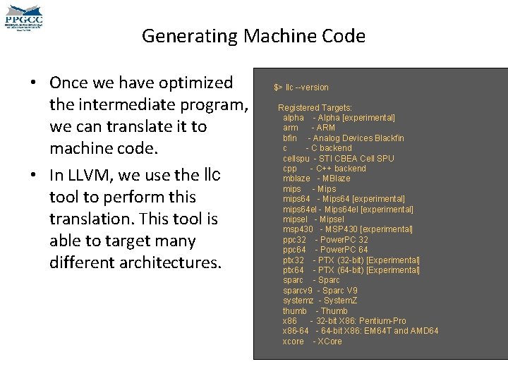
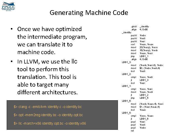
Generating Machine Code • Once we have optimized the intermediate program, we can translate it to machine code. • In LLVM, we use the llc tool to perform this translation. This tool is able to target many different architectures. $> llc --version Registered Targets: alpha - Alpha [experimental] arm - ARM bfin - Analog Devices Blackfin c - C backend cellspu - STI CBEA Cell SPU cpp - C++ backend mblaze - MBlaze mips - Mips mips 64 - Mips 64 [experimental] mips 64 el - Mips 64 el [experimental] mipsel - Mipsel msp 430 - MSP 430 [experimental] ppc 32 - Power. PC 32 ppc 64 - Power. PC 64 ptx 32 - PTX (32 -bit) [Experimental] ptx 64 - PTX (64 -bit) [Experimental] sparc - Sparc sparcv 9 - Sparc V 9 systemz - System. Z thumb - Thumb x 86 - 32 -bit X 86: Pentium-Pro x 86 -64 - 64 -bit X 86: EM 64 T and AMD 64 xcore - XCore

Generating Machine Code • Once we have optimized the intermediate program, we can translate it to machine code. • In LLVM, we use the llc tool to perform this translation. This tool is able to target many different architectures. $> clang -c -emit-llvm identity. c -o identity. bc $> opt -mem 2 reg identity. bc -o identity. opt. bc $> llc -march=x 86 identity. opt. bc -o identity. x 86 . globl. align _identity: pushl xorl movl jmp. align LBB 1_3: movl incl LBB 1_2: cmpl jl incl LBB 1_1: cmpl movl jl jmp LBB 1_6: movl incl LBB 1_5: cmpl jl popl ret _identity 4, 0 x 90 %ebx %edi %esi %eax, %eax 20(%esp), %ecx 16(%esp), %edx %eax, %esi LBB 1_1 4, 0 x 90 (%edx, %esi, 4), %ebx $0, (%ebx, %edi, 4) %edi %ecx, %edi LBB 1_3 %esi %ecx, %esi %eax, %edi LBB 1_2 LBB 1_5 (%edx, %eax, 4), %esi $1, (%esi, %eax, 4) %eax %ecx, %eax LBB 1_6 %esi %edi %ebx

A Bit of History • Some of the first code optimizations were implemented only locally • Fortran was one of the first programming languages to be optimized by a compiler • The LLVM infra-structure was implemented by Chris Lattner, during his Ph. D, at UIUC • Kam, J. B. and J. D. Ullman, "Monotone Data Flow Analysis Frameworks", Actal Informatica 7: 3 (1977), pp. 305 -318 • Kildall, G. "A Unified Approach to Global Program Optimizations", ACM Symposium on Principles of Programming Languages (1973), pp. 194 -206 • Lattner, C. , and Adve, V. , "LLVM: A Compilation Framework for Lifelong Program Analysis & Transformation", CGO, pp. 75 -88 (2004)