Continuum HartreeFock Random Phase Approximation Description of Isovector

Continuum Hartree-Fock Random Phase Approximation Description of Isovector Giant Dipole Resonance in 28 O, 60 Ca and 80 Zr. Emilian Nica Texas A&M University Advisor: Dr. Shalom Shlomo 1

Plan Introduction I. a. b. c. d. Theory II. a. b. c. d. e. III. Overview Collective Modes Isovector Giant Dipole Resonance Collective Motion Models Overview Hartree-Fock Mean-Field Approximation Nucleon-nucleon Interaction Random Phase Approximation Nuclear Response Results and Discussion 2

Part I Introduction 3

Overview n General Remarks ¨ The present discussion deals with the study of the Isovector Giant Dipole Resonance (IVGDR) in symmetric (80 Zr) and neutron-rich (28 O, 60 Ca) nuclei. ¨ The goal of our calculations was to determine whether the small peaks in the RPA response function were indeed due to low-energy resonance effects or to particle emission threshold energies. ¨ We used a Hartree-Fock (HF) Continuum Random Phase Approximation (CRPA) to determine the nuclear response of the three nuclei under study. ¨ The highly accurate HF-CRPA was applied to account for particle excitation into the continuum and to exclude the most common sources of error. 4

Collective Modes n General Description ¨ There are several collective modes in nuclei. A few are illustrated below. Monopole Dipole Quadrupole L=0 L=1 L=2 Isoscalar ( T=0) Isovector ( T=1) ¨ In the isoscalar case, the neutron and proton ensembles oscillate in phase (i. e. dashed line). For the isovector, the neutrons and protons oscillate out of phase. 5

Isovector Giant Dipole Resonance n Brief History The Isovector Giant Dipole Resonance (IVGDR) was the first collective motion seen in nuclei. It was discovered in 1947 by G. C. Baldwin and G. S. Klaiber. ¨ This was done by studying the photon absorption cross section for different nuclei. The giant resonance corresponds to the prominent peak in the graph below. ¨ 6

Collective Motion Models n Liquid Drop Model In the Liquid Drop model the IVGDR is described as the oscillation of the neutron liquid against the proton liquid with a restoring force related to the neutron-proton interaction. ¨ The neutron density is given by ¨ and the proton density is given by In the expressions above ρ0 n and ρ0 p are the neutron and proton saturation densities respectively , 2ε is the small amplitude of the oscillation and is the oscillating frequency. n Microscopic Description In the microscopic treatment of collective motion the nuclear wave function is described as a linear combination of particle-hole excitations. ¨ We used the Hartree-Fock (HF) based Continuum Random Phase Approximation (CRPA) to calculate the response function of the IVGDR in symmetric (80 Zr) and neutron-rich nuclei (28 O and 60 Ca). ¨ 7

Part II Theory 8

Overview n Microscopic Model ¨ The microscopic model involves the use of HF-CRPA calculations to describe the collective motion in nuclei. In essence, its use involves the collective effect of single-particle excitations on the structure of the nucleus. ¨ The HF-CRPA calculations model the collective motion through changes in the ground-state nuclear wave function induced by particle-hole excitations. ¨ The collective aspect of the motion is accounted for by considering all possible single-particle excitations and the overall effect these have on the nuclear properties. ¨ Our calculations were based on a Green’s function HF-CRPA. This allows for solutions in coordinate space as opposed to configuration space and for a simplification of the procedure. 9

Hartree-Fock Mean-Field Approximation n General Remarks ¨ The Hartree-Fock Mean-Field Approximation is a method used to solve the nuclear many-body problem. ¨ The Hartree-Fock calculations allow us to determine the nuclear groundstate wave function and energy. ¨ The Hartree-Fock method and results provide a basis (i. e. wave function , Hamiltonian and single-particle energies) for the introduction of particle -hole excitations in the RPA. 10

Hartree-Fock Mean-Field Approximation n n Hamiltonian Operator ¨ The total Hamiltonian of the many-body nuclear system can be written as a sum of the single-particle kinetic energies and two-body interactions (potentials) ¨ V is the short-range, nucleon-nucleon interaction and it is written here in general form. The potential V can be chosen a specific form (i. e. Skyrme interaction). Mean-Field Approximation ¨ The many-body Schrodinger equation is difficult to solve. We will use a mean-field approximation to considerably simplify our models. In a mean-field approximation each particle moves independently of other nucleons in a central potential U representing the interaction of a nucleon with all the other nucleons. 11

n Slater Determinant ¨ Because of the antisymmetrization of the overall nuclear wave function Φ 0 in the mean-field approximation, it can be written as a determinant known as the Slater determinant The arguments 1, 2…, A above denote the coordinates of the particles (position and spin) while λ are the single-particle wave functions. ¨ By interchanging any two rows the sign of the wave function will change (i. e. antisymmetry). 12

n Variational Principle ¨ By applying the variational principle to the expectation value of the Hamiltonian and normalizing through the use of Lagrange multipliers we obtained after some calculations the HF equations ¨ The HF equations can be solved in an iterative way by “guessing” an initial set of wave functions λ, solving the equations above for new single-particle wave functions and repeating the process until convergence (i. e. ελ converge). 13

Nucleon-nucleon interaction ¨ In our calculation we used a simplified Skyrme type effective nucleon interaction given by where the parameters t 0, t 3 and α are obtained by fitting the HF results to experimental data. ¨ In our calculations we have used the values of: t 0=-1600 Me. V fm 3 t 3=12500 Me. V fm 4 α=1/3 14

Random Phase Approximation n Microscopic Treatment In the microscopic treatment of collective vibrations within the RPA method the new wave function is a linear combination of all possible single-particle excitations. ¨ In our treatment of the IVGDR we will use a Green’s function formalism instead of a “standard” RPA procedure (i. e. configuration space). ¨ n Linear Response Theory ¨ The bare particle-hole Green’s function is defined as In the preceding equation, h is the occupied single-particle wave function with the corresponding single-particle energy εh, H 0 is the HF Hamiltonian and is the excitation energy of the nucleus. 15

Random Phase Approximation ¨ The RPA Green’s function is obtained from The term Vph in the expression above stands for the particle-hole interaction and it is directly linked to the RPA procedure since it represents the additional interaction introduced by single-particle excitations. ¨ The formalism must account for the possibility of the excitation of a particle beyond the binding energy threshold (i. e. into the continuum). 16

Random Phase Approximation n Continuum Effects ¨ Because of the possibility of particle excitation into the continuum the single-particle Green’s function is obtained from ulj is the regular solution to the HF Hamiltonian and vlj is the irregular solution (i. e. numerical solution starting from a low r to r and vice versa). The r and r stand for lesser and greater of r and r’, respectively, while W is the Wronskian ¨ The boundary condition for the irregular solution at r is: For positive energies E, this describes an outgoing wave asymptotically. ¨ We note that in our calculations we have used a very small value for the smearing parameter : /2=0. 01 Me. V. ¨ 17

Nuclear Response n General Remarks ¨ We define a scattering operator F such as ¨ The nuclear response is given by the Strength Function S(E): where and denote the ground and excited states, respectively. ¨ In the Green’s function formalism ¨ Another useful value is the transition density. In our case it can be obtained using the relation 18

Part III Results and Discussion 19

Results Figure 1. The IVGDR free and RPA response functions for 60 Ca (in arbitrary units). 21

Results Figure 2. Similar to Figure 1 for 28 O. 22

Results Figure 3. Similar to Figure 1 for the symmetric nucleus 80 Zr. 23

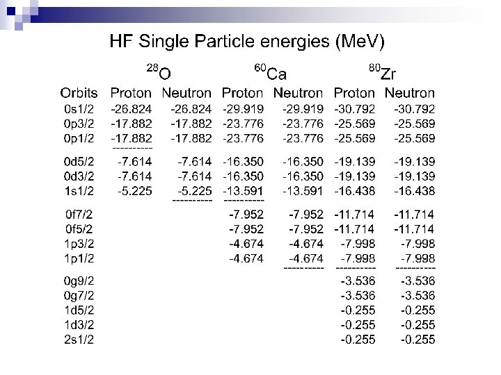
of the free (top) and RPA (bottom) of the response functions for 28 O, 60 Ca and 80 Zr. Discussion n For a resonance has a peak at a resonance energy E=ER, and decreases with E, going through zero at ER. n Example 60 Ca: (i) (iii) (iv) Threshold energies: Sn=4. 674 Me. V, Sp=13. 591 Me. V. The sharp peaks at 8. 398, 8. 917 and 11. 676 Me. V are due to proton bound to bound particle-hole excitations π0 d -> π0 f, π1 s -> π1 p and π0 d -> π1 p, respectively. The neutron particle-hole excitation are all to the continuum. Note threshold effect of enhancement in above 4. 674 Me. V and at around 6 Me. V. In the RPA excitation strength ( ) we observe the collective IVGDR above 11 Me. V with threshold enhancement at low excitation energies. 24

Summary We have carried out the HF-based-Continuum RPA calculation of the IVGDR response function for the symmetric nucleus 80 Zr and the neutron-rich nuclei 28 O and 60 Ca. We have demonstrated the important threshold effect of enhancement in the IVGDR excitation strength at low excitation energies in neutronrich nuclei associated with loosely bound orbits. In 80 Zr, due to the large single-particle separation energies, the corresponding threshold enhancements in the excitation strength are negligible. In common RPA calculations with discretized continuum these strength enhancements incorrectly appear as low-lying excited states, also termed soft dipole modes. 25

Acknowledgments Work done at: 26

Work supported by: 27

Hartree-Fock Mean-Field Approximation n Antisymmetry ¨ The Pauli exclusion principle states that no two identical fermions can occupy the same state. A consequence of this is that interchanging the positions of 2 particles will change the sign of the overall wave function. ¨ Let Ψab(r 12) be a wavefunction of two particles with r 12 the distance between the particles and a , b the occupied orbits. The Pauli exclusion principle implies that Ψab(r 12) → 0 as r 12 → 0. ¨ If Ψab(r 12)= Ψa(r 1) Ψb (r 2) it is not necessary that the above condition is respected. A better expression would be , which vanishes when r 1=r 2. 28

Random Phase Approximation n General Remarks: ¨ The Random Phase Approximation (RPA) is a method to describe excitations of ground state particles. For a single particle excitation the RPA shifts a particle from its ground state into a higher energy state. A schematic illustration of this is shown below. ¨ In a Slater Determinant formalism this corresponds to the annihilation of one state (i. e. a row) and the creation of a new state in place of the previous one. The energy of the system is the eigenvalue corresponding to the new nuclear wave function. 29