Continuous Random Variables Lecture 22 Section 7 5

Continuous Random Variables Lecture 22 Section 7. 5. 4 Mon, Feb 25, 2008

Random Variables Random variable n Discrete random variable n Continuous random variable n

Continuous Probability Distribution Functions Continuous Probability Distribution Function (pdf) – For a random variable X, it is a function with the property that the area below the graph of the function between any two points a and b equals the probability that a ≤ X ≤ b. n Remember, AREA = PROPORTION = PROBABILITY n

Example The TI-83 will return a random number between 0 and 1 if we enter rand press ENTER. n These numbers have a uniform distribution from 0 to 1. n Let X be the random number returned by the TI-83. n

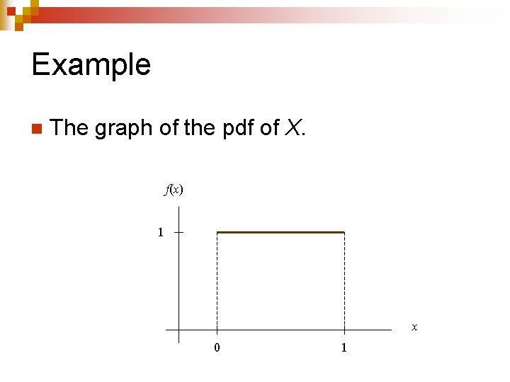
Example n The graph of the pdf of X. f(x) 1 x 0 1

Example n What is the probability that the random number is at least 0. 3?

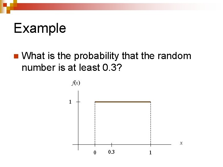
Example n What is the probability that the random number is at least 0. 3? f(x) 1 x 0 0. 3 1

Example n What is the probability that the random number is at least 0. 3? f(x) 1 x 0 0. 3 1

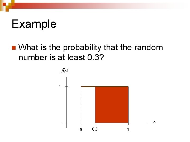
Example n What is the probability that the random number is at least 0. 3? f(x) 1 x 0 0. 3 1

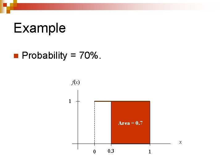
Example n Probability = 70%. f(x) 1 Area = 0. 7 x 0 0. 3 1

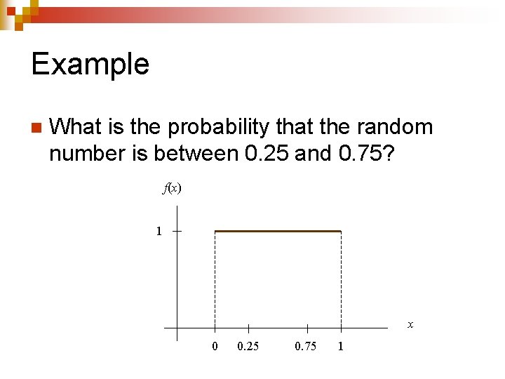
Example n What is the probability that the random number is between 0. 25 and 0. 75? f(x) 1 x 0 0. 25 0. 75 1

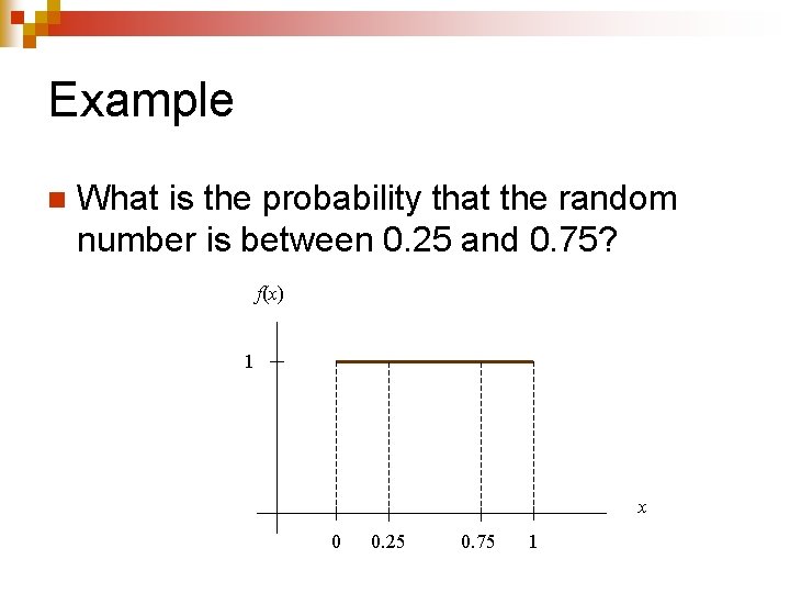
Example n What is the probability that the random number is between 0. 25 and 0. 75? f(x) 1 x 0 0. 25 0. 75 1

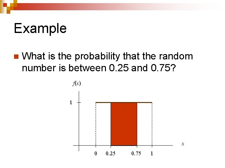
Example n What is the probability that the random number is between 0. 25 and 0. 75? f(x) 1 x 0 0. 25 0. 75 1

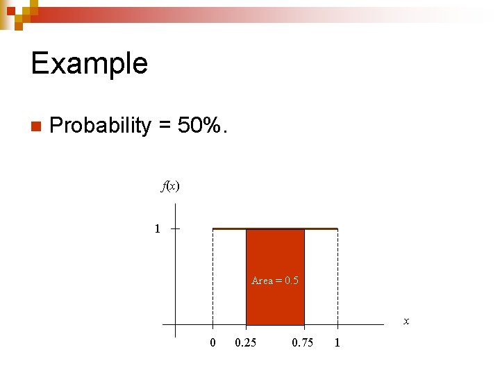
Example n Probability = 50%. f(x) 1 Area = 0. 5 x 0 0. 25 0. 75 1

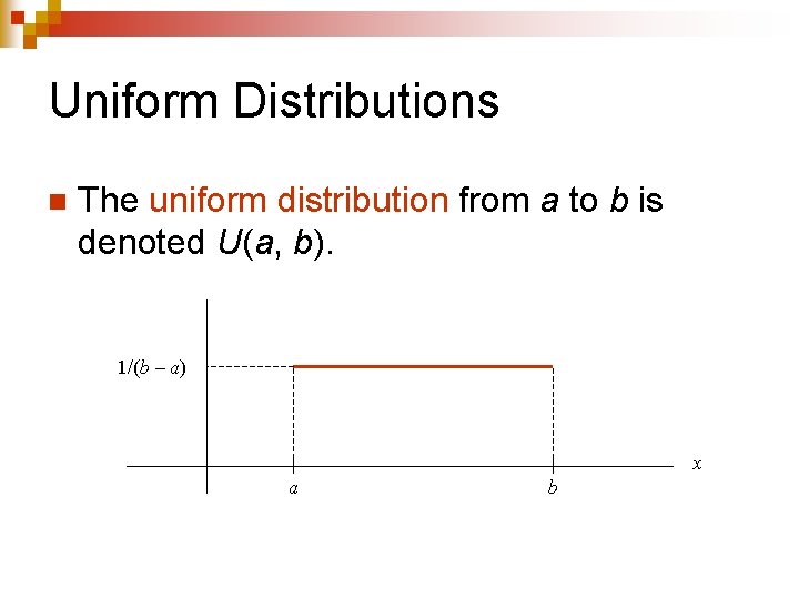
Uniform Distributions n The uniform distribution from a to b is denoted U(a, b). 1/(b – a) x a b

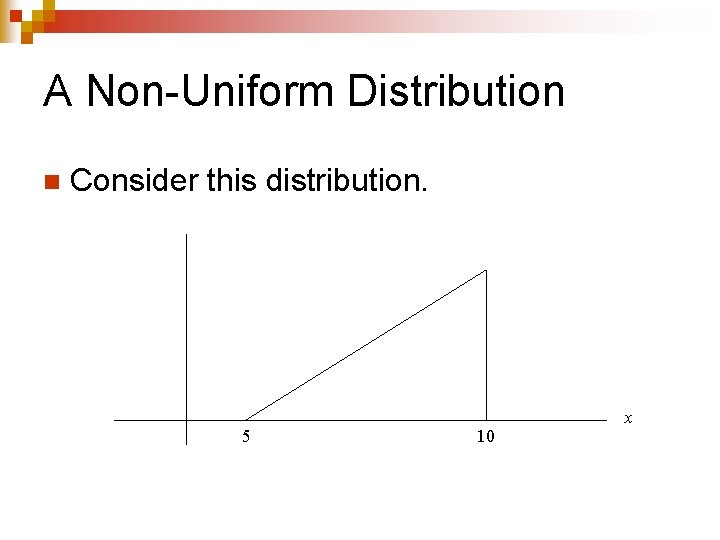
A Non-Uniform Distribution n Consider this distribution. 5 10 x

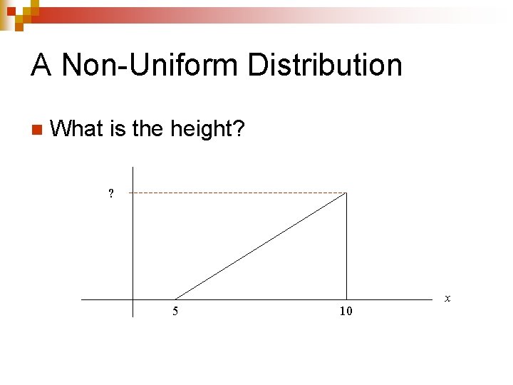
A Non-Uniform Distribution n What is the height? ? 5 10 x

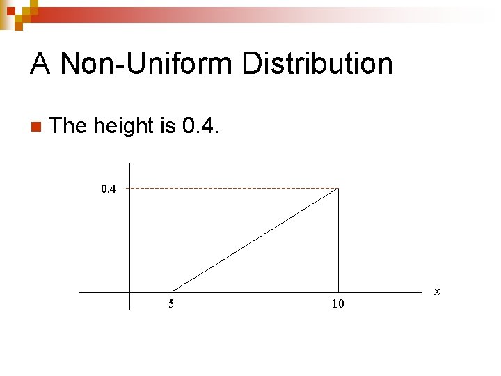
A Non-Uniform Distribution n The height is 0. 4 5 10 x

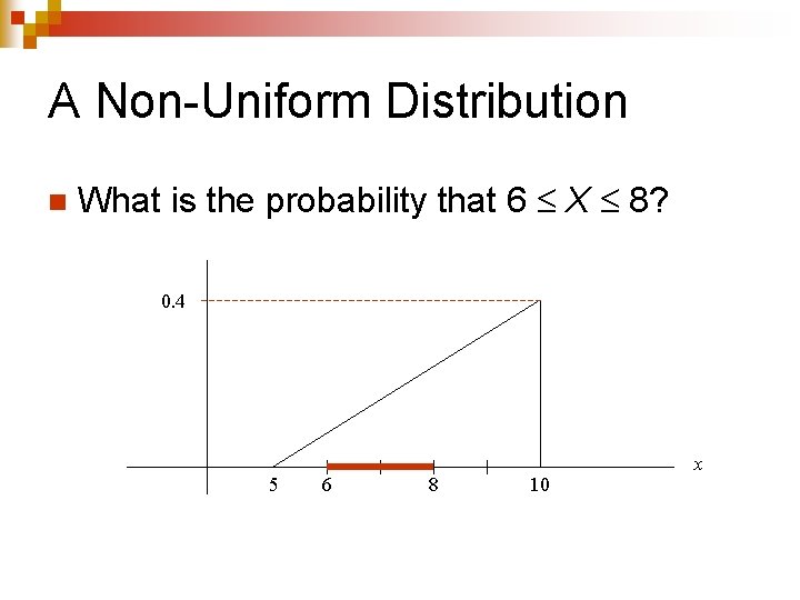
A Non-Uniform Distribution n What is the probability that 6 X 8? 0. 4 5 6 8 10 x

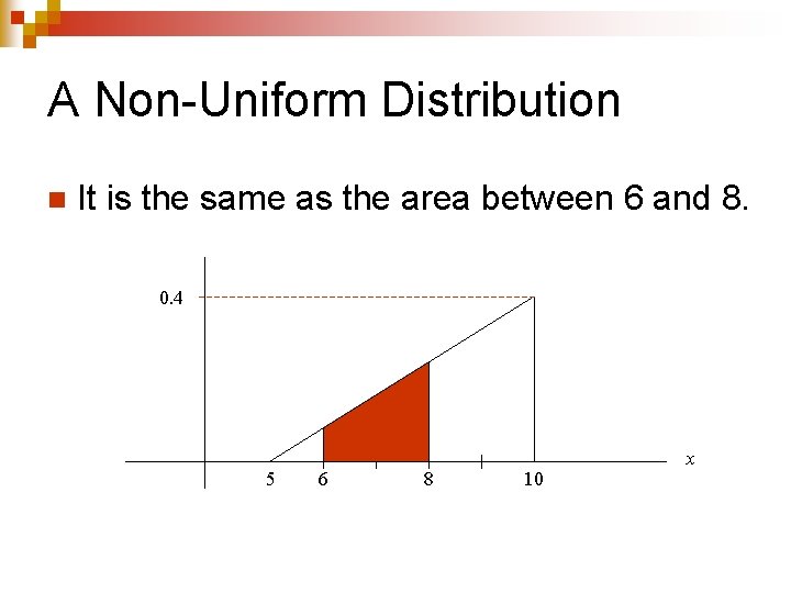
A Non-Uniform Distribution n It is the same as the area between 6 and 8. 0. 4 5 6 8 10 x

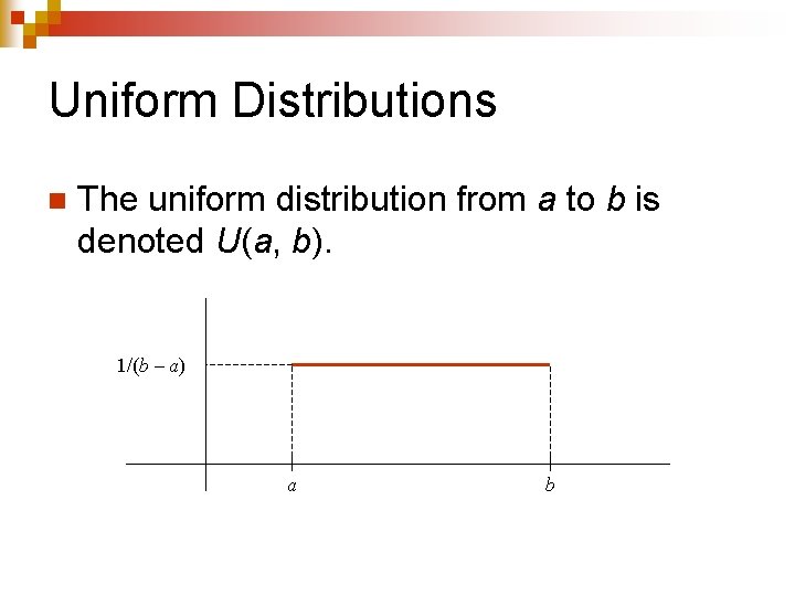
Uniform Distributions n The uniform distribution from a to b is denoted U(a, b). 1/(b – a) a b

Hypothesis Testing (n = 1) n An experiment is designed to determine whether a random variable X has the distribution U(0, 1) or U(0. 5, 1. 5). ¨ H 0: X is U(0, 1). ¨ H 1: X is U(0. 5, 1. 5). n One value of X is sampled (n = 1).

Hypothesis Testing (n = 1) n An experiment is designed to determine whether a random variable X has the distribution U(0, 1) or U(0. 5, 1. 5). ¨ H 0: X is U(0, 1). ¨ H 1: X is U(0. 5, 1. 5). One value of X is sampled (n = 1). n If X is more than 0. 75, then H 0 will be rejected. n

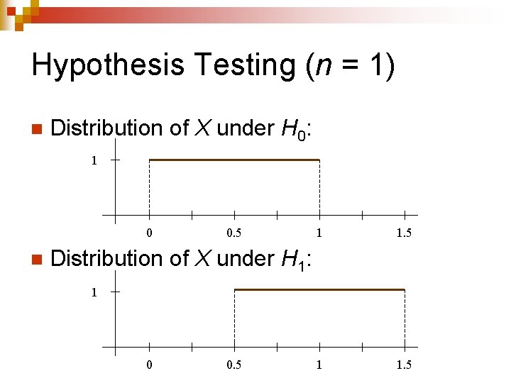
Hypothesis Testing (n = 1) n Distribution of X under H 0: 1 0 n 0. 5 1 1. 5 Distribution of X under H 1: 1 0 0. 5

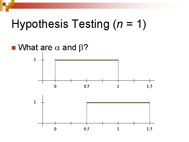
Hypothesis Testing (n = 1) n What are and ? 1 0 0. 5 1 1. 5 1

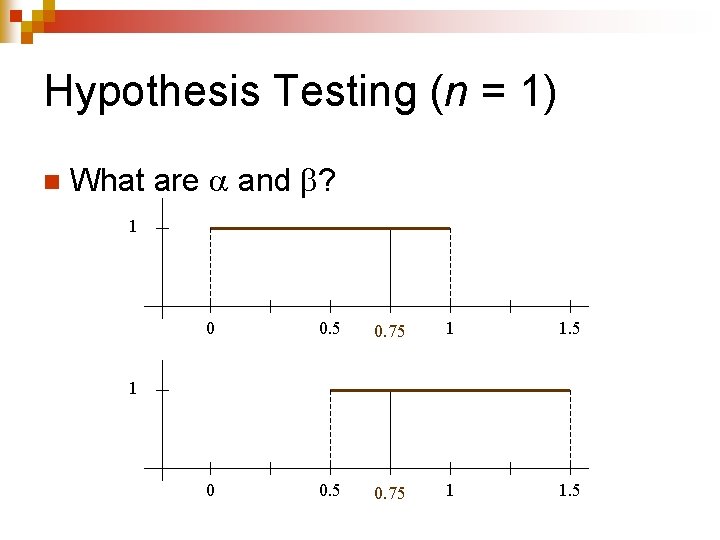
Hypothesis Testing (n = 1) n What are and ? 1 0 0. 5 0. 75 1 1. 5 1

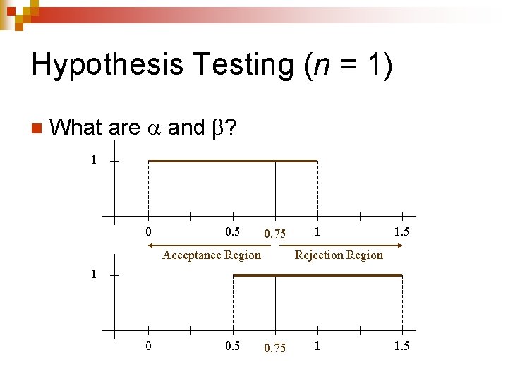
Hypothesis Testing (n = 1) n What are and ? 1 0 0. 5 0. 75 Acceptance Region 1 1. 5 Rejection Region 1 0 0. 5 0. 75 1 1. 5

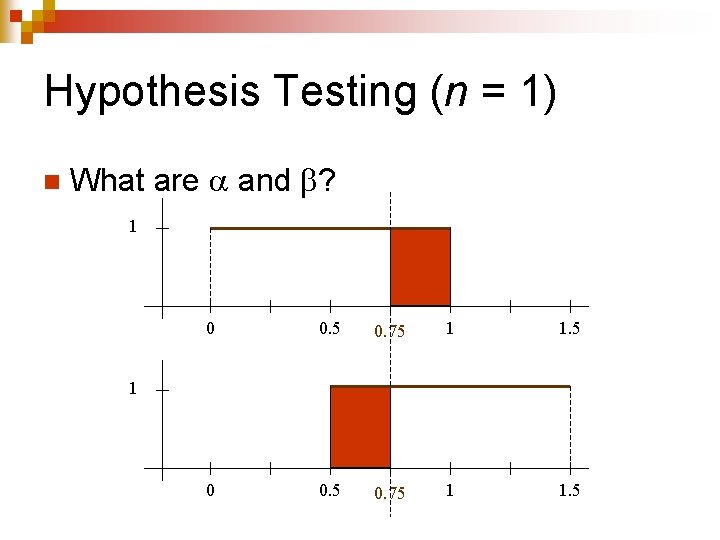
Hypothesis Testing (n = 1) n What are and ? 1 0 0. 5 0. 75 1 1. 5 1

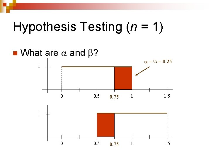
Hypothesis Testing (n = 1) n What are and ? = ¼ = 0. 25 1 0 0. 5 0. 75 1 1. 5 1

Hypothesis Testing (n = 1) n What are and ? = ¼ = 0. 25 1 0. 5 0. 75 1 1. 5 = ¼ = 0. 25 0

Example Now suppose we use the TI-83 to get two random numbers from 0 to 1, and then add them together. n Let X 2 = the average of the two random numbers. n What is the pdf of X 2? n

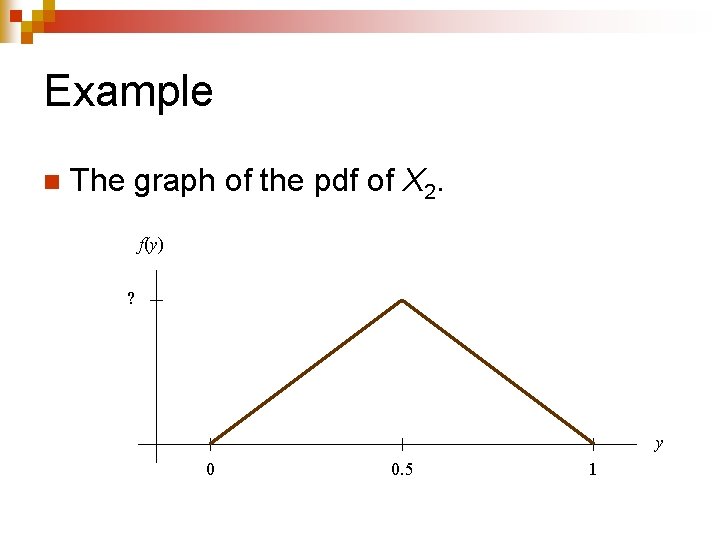
Example n The graph of the pdf of X 2. f(y) ? y 0 0. 5 1

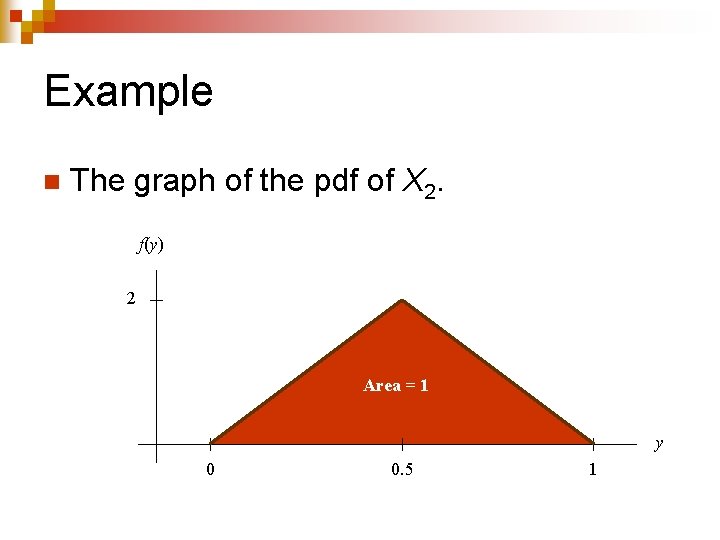
Example n The graph of the pdf of X 2. f(y) 2 Area = 1 y 0 0. 5 1

Example n What is the probability that X 2 is between 0. 25 and 0. 75? f(y) 2 y 0 0. 25 0. 75 1

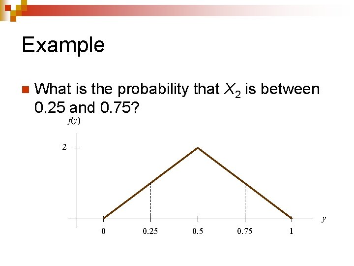
Example n What is the probability that X 2 is between 0. 25 and 0. 75? f(y) 2 y 0 0. 25 0. 75 1

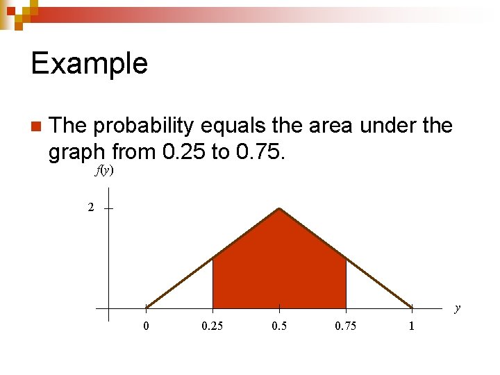
Example n The probability equals the area under the graph from 0. 25 to 0. 75. f(y) 2 y 0 0. 25 0. 75 1

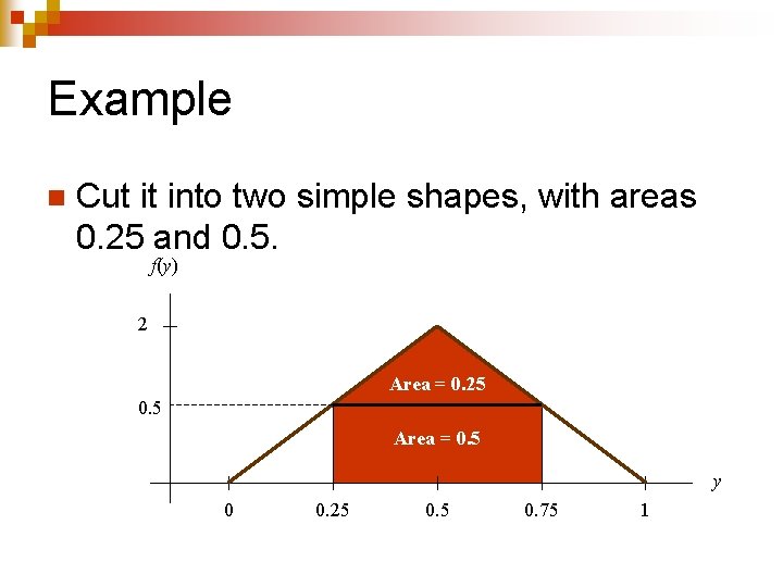
Example n Cut it into two simple shapes, with areas 0. 25 and 0. 5. f(y) 2 Area = 0. 25 0. 5 Area = 0. 5 y 0 0. 25 0. 75 1

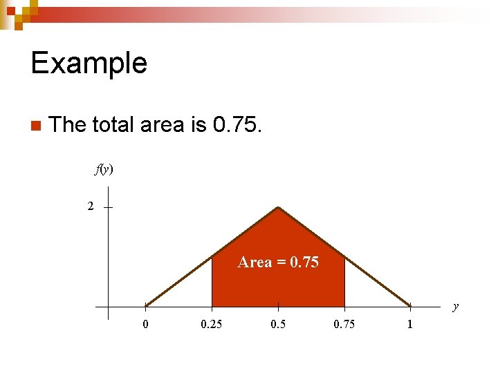
Example n The total area is 0. 75. f(y) 2 Area = 0. 75 y 0 0. 25 0. 75 1

Hypothesis Testing (n = 2) n An experiment is designed to determine whether a random variable X has the distribution U(0, 1) or U(0. 5, 1. 5). ¨ H 0: X is U(0, 1). ¨ H 1: X is U(0. 5, 1. 5). n n n Two values of X are sampled (n = 2). Let X 2 be the average. If X 2 is more than 0. 75, then H 0 will be rejected.

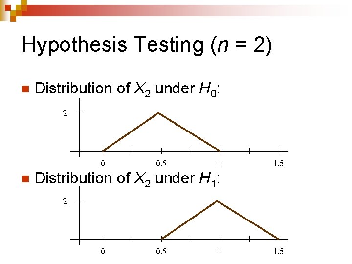
Hypothesis Testing (n = 2) n Distribution of X 2 under H 0: 2 0 n 0. 5 1 1. 5 Distribution of X 2 under H 1: 2 0 0. 5 1 1. 5

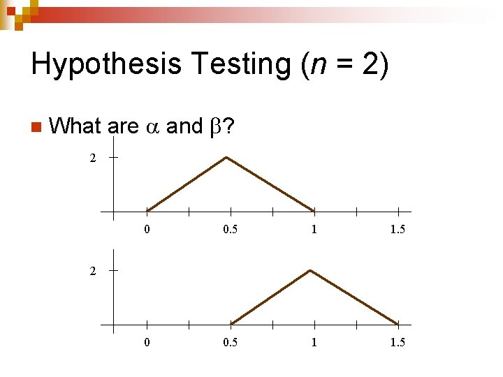
Hypothesis Testing (n = 2) n What are and ? 2 0 0. 5 1 1. 5 2

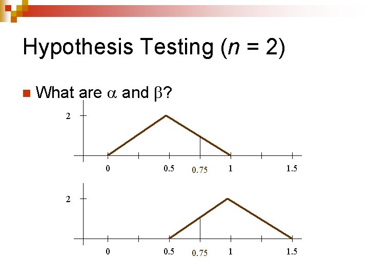
Hypothesis Testing (n = 2) n What are and ? 2 0 0. 5 0. 75 1 1. 5 2

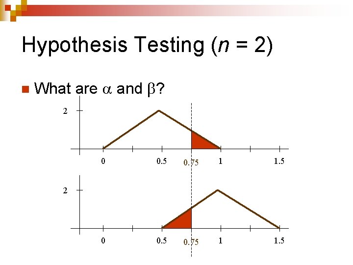
Hypothesis Testing (n = 2) n What are and ? 2 0 0. 5 0. 75 1 1. 5 2

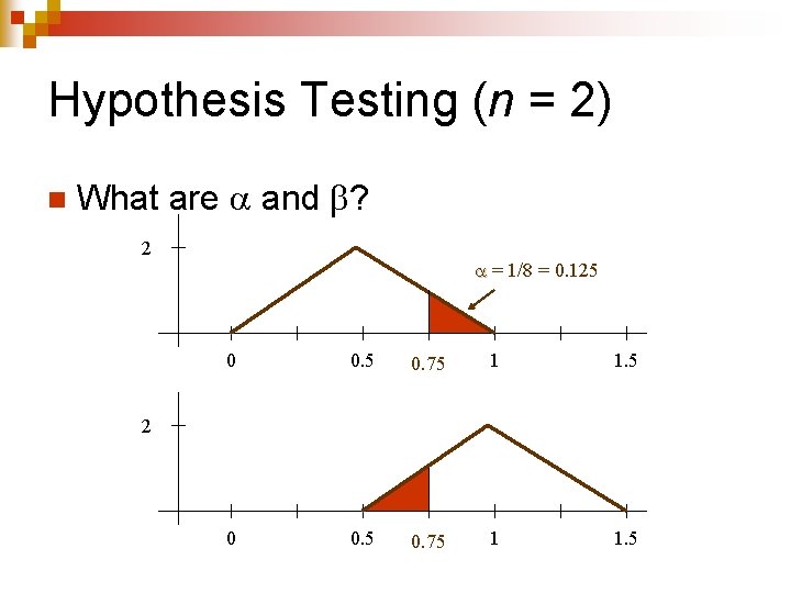
Hypothesis Testing (n = 2) n What are and ? 2 = 1/8 = 0. 125 0 0. 5 0. 75 1 1. 5 2

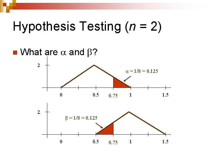
Hypothesis Testing (n = 2) n What are and ? 2 = 1/8 = 0. 125 0 2 0. 5 0. 75 1 1. 5 = 1/8 = 0. 125 0 0. 5

Conclusion n By increasing the sample size, we can lower both and simultaneously.