Contingency Tables cross tabs Generally used when variables

Contingency Tables (cross tabs) Ø Generally used when variables are nominal and/or ordinal l Ø Even here, should have a limited number of variable attributes (categories) Some find these very intuitive…others struggle l It is very easy to misinterpret these critters

Interpreting a Contingency Table Ø WHAT IS IN THE INDIVIDUAL CELLS? l The number of cases that fit in that particular cell • In other words, frequencies (number of cases that fit criteria) l For small tables, and/or small sample sizes, it may be possible to detect relationships by “eyeballing” frequencies. For most. . • Convert to Percentages: a way to standardize cells and make relationships more apparent

Example 1 Ø Random sample of UMD students to examine political party membership l Are UMD students more likely to belong to particular political parties? • • l Democrat Republican Independent Green (N=40 UMD students)

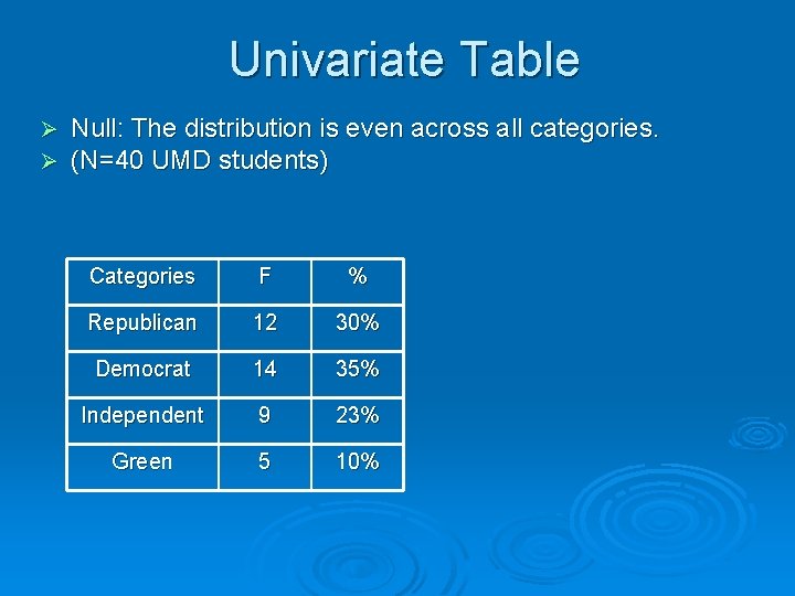
Univariate Table Ø Ø Null: The distribution is even across all categories. (N=40 UMD students) Categories F % Republican 12 30% Democrat 14 35% Independent 9 23% Green 5 10%

Example 2 Ø A survey of 10, 000 U. S. residents Ø Is one’s political view related to attitudes towards police? What are the DV and IV? Ø Convention for bivariate tables l l l The IV is on the top of the table (dictates columns) The DV is on the side (dictates rows).

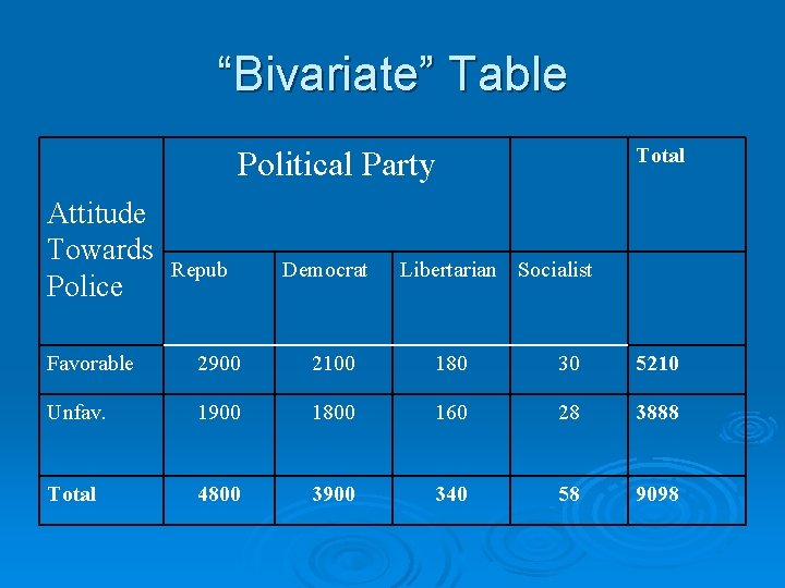
“Bivariate” Table Total Political Party Attitude Towards Police Repub Democrat Libertarian Socialist Favorable 2900 2100 180 30 5210 Unfav. 1900 1800 160 28 3888 Total 4800 3900 340 58 9098

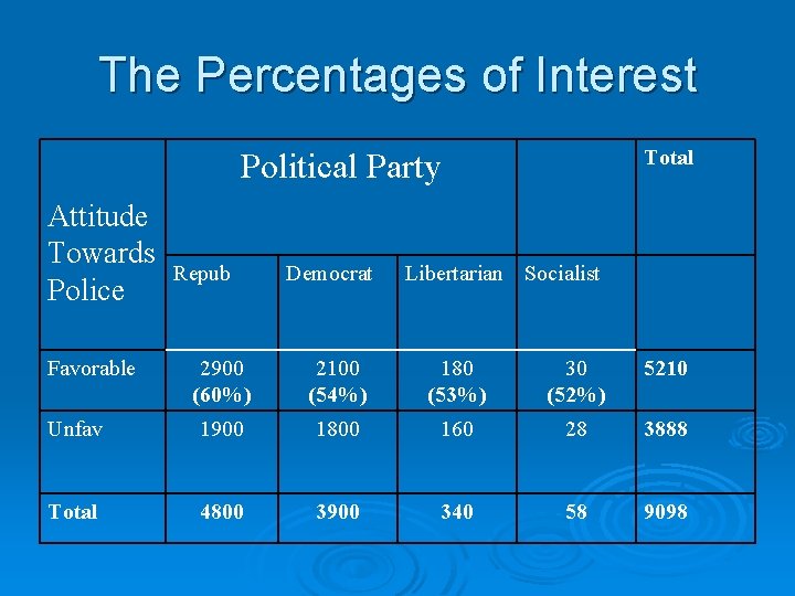
The Percentages of Interest Total Political Party Attitude Towards Police Favorable Repub Democrat Libertarian Socialist 2900 (60%) 2100 (54%) 180 (53%) 30 (52%) 5210 Unfav 1900 1800 160 28 3888 Total 4800 3900 340 58 9098

The Test Statistic for Contingency Tables Ø Chi Square, or χ2 l Calculation • Observed frequencies (your sample data) • Expected frequencies (UNDER NULL) l l Intuitive: how different are the observed cell frequencies from the expected cell frequencies Degrees of Freedom: • 1 -way = K-1 • 2 -way = (# of Rows -1) (# of Columns -1)

“One-Way” CHI SQUARE Ø The most simple form of the Chi square is the one-way Chi square test Ø For Univariate Table • Do frequencies observed differ significantly from an even distribution? • Null hypothesis: there are no differences across the categories in the population

Chi Square: Steps 1. 2. 3. 4. Find the expected (under null hypothesis) cell frequencies Compare expected & observed frequencies cell by cell If null hypothesis is true, expected and observed frequencies should be close in value Greater the difference between the observed and expected frequencies, the greater the possibility of rejecting the null

Calculating χ2 Ø χ2 l = ∑ [(fo - fe)2 /fe] Where Fe= Row Marginal X Column Marginal N So, for each cell, calculate the difference between the actual frequencies (“observed”) and what frequencies would be expected if the null was true (“expected”). Square, and divide by the expected frequency. Ø Add the results from each cell. Ø

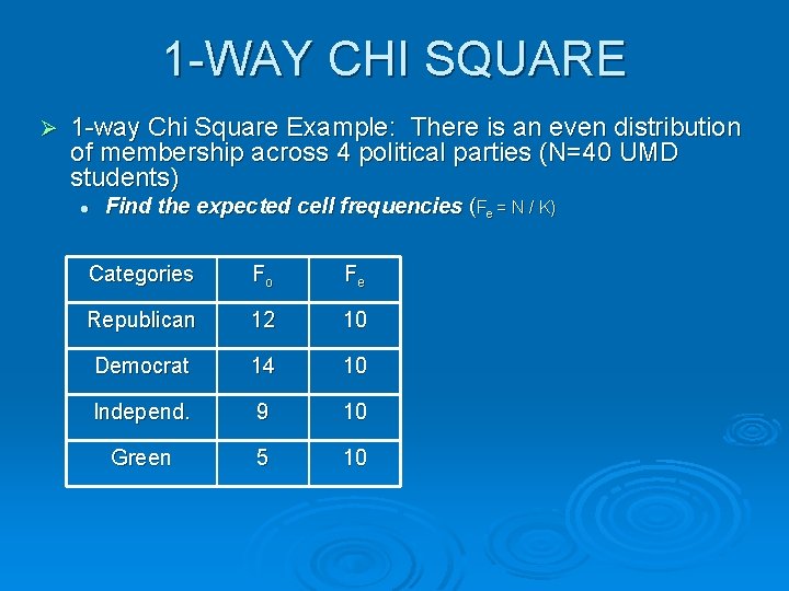
1 -WAY CHI SQUARE Ø 1 -way Chi Square Example: There is an even distribution of membership across 4 political parties (N=40 UMD students) l Find the expected cell frequencies (Fe = N / K) Categories Fo Fe Republican 12 10 Democrat 14 10 Independ. 9 10 Green 5 10

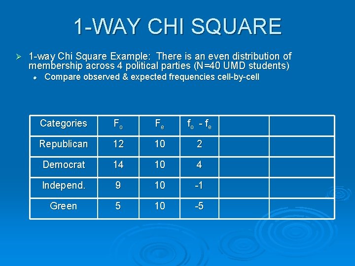
1 -WAY CHI SQUARE Ø 1 -way Chi Square Example: There is an even distribution of membership across 4 political parties (N=40 UMD students) l Compare observed & expected frequencies cell-by-cell Categories Fo Fe fo - f e Republican 12 10 2 Democrat 14 10 4 Independ. 9 10 -1 Green 5 10 -5

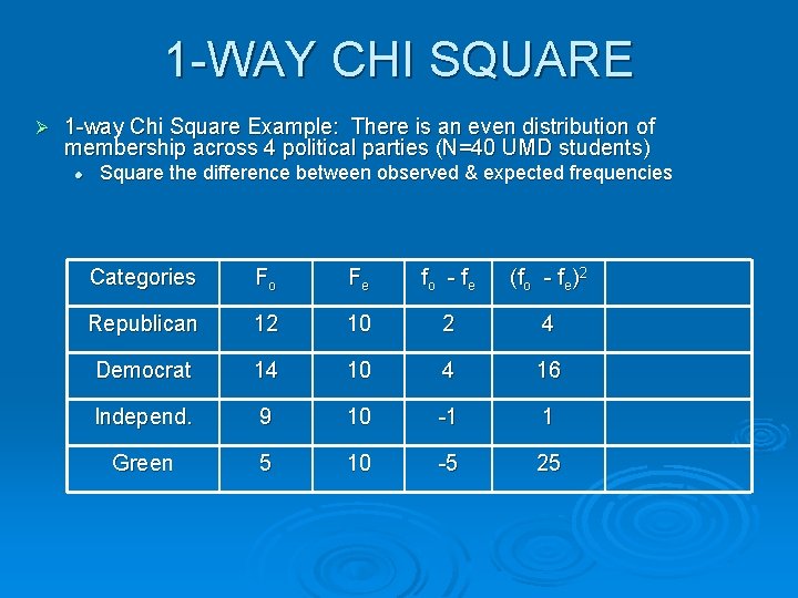
1 -WAY CHI SQUARE Ø 1 -way Chi Square Example: There is an even distribution of membership across 4 political parties (N=40 UMD students) l Square the difference between observed & expected frequencies Categories Fo Fe fo - f e (fo - fe)2 Republican 12 10 2 4 Democrat 14 10 4 16 Independ. 9 10 -1 1 Green 5 10 -5 25

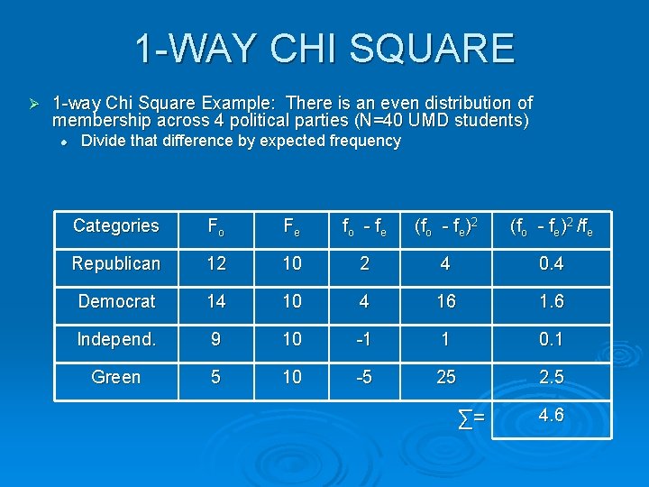
1 -WAY CHI SQUARE Ø 1 -way Chi Square Example: There is an even distribution of membership across 4 political parties (N=40 UMD students) l Divide that difference by expected frequency Categories Fo Fe fo - f e (fo - fe)2 /fe Republican 12 10 2 4 0. 4 Democrat 14 10 4 16 1. 6 Independ. 9 10 -1 1 0. 1 Green 5 10 -5 25 2. 5 ∑= 4. 6

Interpreting Chi-Square Ø Chi-square has no intuitive meaning, it can range from zero to very large l As with other test statistics, the real interest is the “p value” associated with the calculated chi-square value • Conventional testing = find χ2 (critical) for stated “alpha” (. 05, . 01, etc. ) l Reject if χ2 (observed) is greater than χ2 (critical) • SPSS: find the exact probability of obtaining the χ2 under the null (reject if less than alpha)

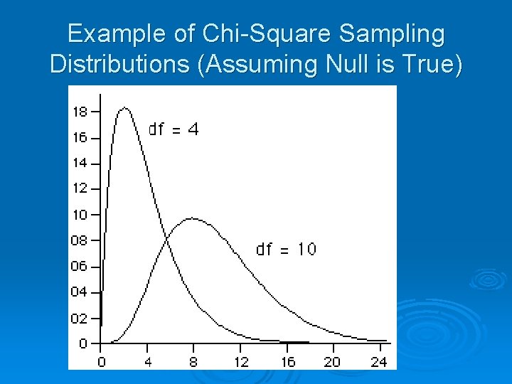
Example of Chi-Square Sampling Distributions (Assuming Null is True)

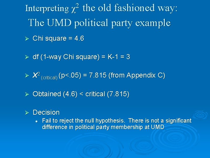
Interpreting χ2 the old fashioned way: The UMD political party example Ø Chi square = 4. 6 Ø df (1 -way Chi square) = K-1 = 3 Ø X 2 (critical) (p<. 05) = 7. 815 (from Appendix C) Ø Obtained (4. 6) < critical (7. 815) Ø Decision l Fail to reject the null hypothesis. There is not a significant difference in political party membership at UMD

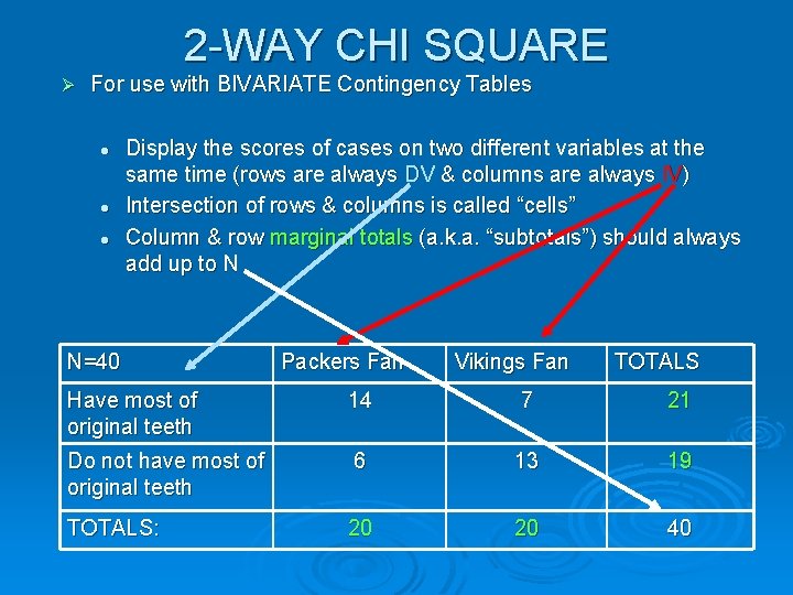
2 -WAY CHI SQUARE Ø For use with BIVARIATE Contingency Tables l l l Display the scores of cases on two different variables at the same time (rows are always DV & columns are always IV) Intersection of rows & columns is called “cells” Column & row marginal totals (a. k. a. “subtotals”) should always add up to N N=40 Packers Fan Vikings Fan TOTALS Have most of original teeth 14 7 21 Do not have most of original teeth 6 13 19 TOTALS: 20 20 40

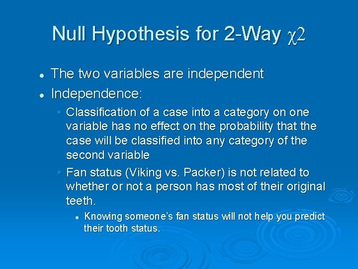
Null Hypothesis for 2 -Way χ2 l l The two variables are independent Independence: • Classification of a case into a category on one variable has no effect on the probability that the case will be classified into any category of the second variable • Fan status (Viking vs. Packer) is not related to whether or not a person has most of their original teeth. l Knowing someone’s fan status will not help you predict their tooth status.

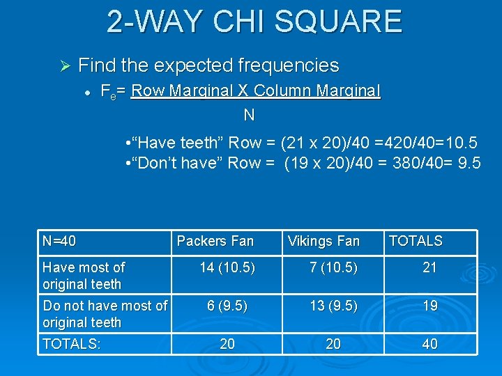
2 -WAY CHI SQUARE Ø Find the expected frequencies l Fe= Row Marginal X Column Marginal N • “Have teeth” Row = (21 x 20)/40 =420/40=10. 5 • “Don’t have” Row = (19 x 20)/40 = 380/40= 9. 5 N=40 Have most of original teeth Do not have most of original teeth TOTALS: Packers Fan Vikings Fan TOTALS 14 (10. 5) 7 (10. 5) 21 6 (9. 5) 13 (9. 5) 19 20 20 40

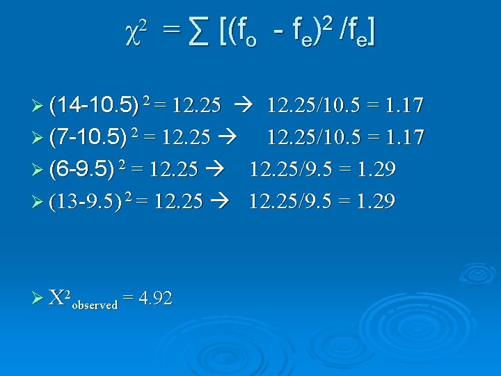
χ = ∑ [(fo 2 Ø (14 -10. 5) 2 = 12. 25 2 fe) /fe] 12. 25/10. 5 = 1. 17 Ø (7 -10. 5) 2 = 12. 25/10. 5 = 1. 17 Ø (6 -9. 5) 2 = 12. 25/9. 5 = 1. 29 Ø (13 -9. 5) 2 = 12. 25/9. 5 = 1. 29 Ø Χ 2 observed = 4. 92

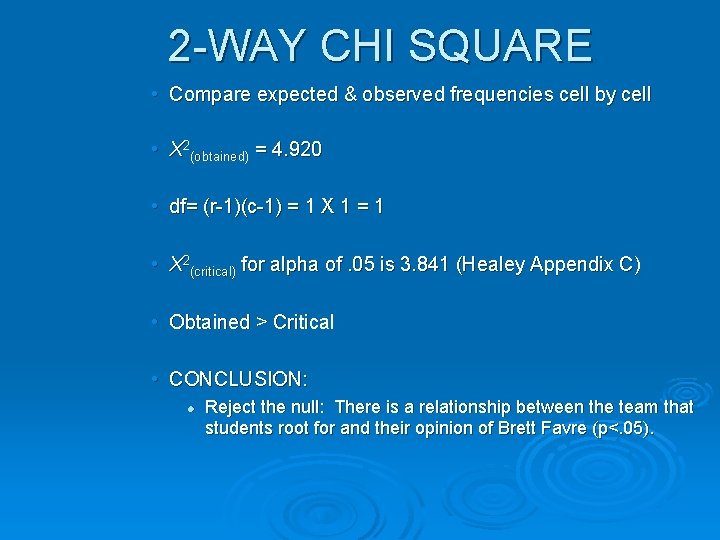
2 -WAY CHI SQUARE • Compare expected & observed frequencies cell by cell • X 2(obtained) = 4. 920 • df= (r-1)(c-1) = 1 X 1 = 1 • X 2(critical) for alpha of. 05 is 3. 841 (Healey Appendix C) • Obtained > Critical • CONCLUSION: l Reject the null: There is a relationship between the team that students root for and their opinion of Brett Favre (p<. 05).

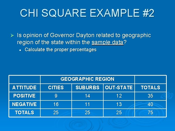
CHI SQUARE EXAMPLE #2 Ø Is opinion of Governor Dayton related to geographic region of the state within the sample data? l Calculate the proper percentages GEOGRAPHIC REGION ATTITUDE CITIES SUBURBS OUT-STATE TOTALS POSITIVE 9 14 12 35 NEGATIVE 16 11 13 40 TOTALS 25 25 25 75

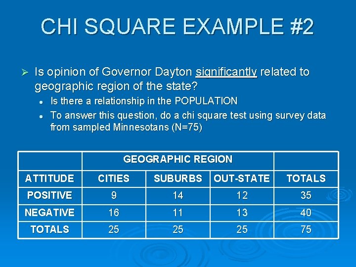
CHI SQUARE EXAMPLE #2 Ø Is opinion of Governor Dayton significantly related to geographic region of the state? l l Is there a relationship in the POPULATION To answer this question, do a chi square test using survey data from sampled Minnesotans (N=75) GEOGRAPHIC REGION ATTITUDE CITIES SUBURBS OUT-STATE TOTALS POSITIVE 9 14 12 35 NEGATIVE 16 11 13 40 TOTALS 25 25 25 75

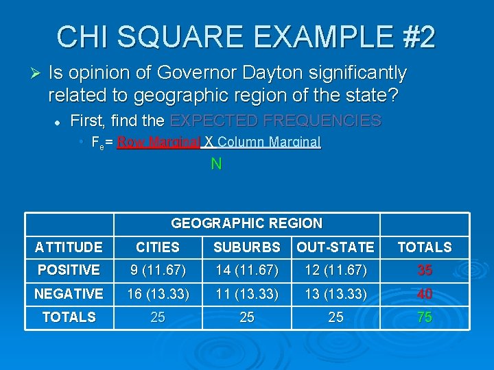
CHI SQUARE EXAMPLE #2 Ø Is opinion of Governor Dayton significantly related to geographic region of the state? l First, find the EXPECTED FREQUENCIES • Fe= Row Marginal X Column Marginal N GEOGRAPHIC REGION ATTITUDE CITIES SUBURBS OUT-STATE TOTALS POSITIVE 9 (11. 67) 14 (11. 67) 12 (11. 67) 35 NEGATIVE 16 (13. 33) 11 (13. 33) 13 (13. 33) 40 TOTALS 25 25 25 75

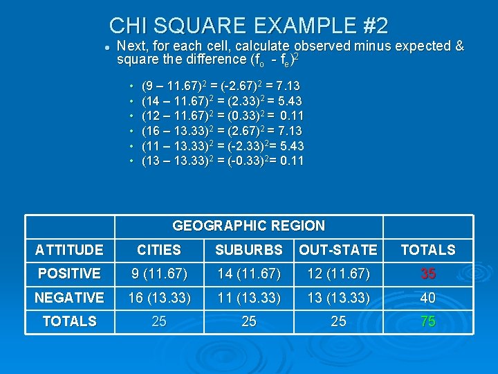
CHI SQUARE EXAMPLE #2 l Next, for each cell, calculate observed minus expected & square the difference (fo - fe)2 • • • (9 – 11. 67)2 = (-2. 67)2 = 7. 13 (14 – 11. 67)2 = (2. 33)2 = 5. 43 (12 – 11. 67)2 = (0. 33)2 = 0. 11 (16 – 13. 33)2 = (2. 67)2 = 7. 13 (11 – 13. 33)2 = (-2. 33)2= 5. 43 (13 – 13. 33)2 = (-0. 33)2= 0. 11 GEOGRAPHIC REGION ATTITUDE CITIES SUBURBS OUT-STATE TOTALS POSITIVE 9 (11. 67) 14 (11. 67) 12 (11. 67) 35 NEGATIVE 16 (13. 33) 11 (13. 33) 13 (13. 33) 40 TOTALS 25 25 25 75

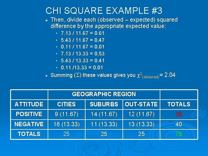
CHI SQUARE EXAMPLE #3 l l Then, divide each (observed – expected) squared difference by the appropriate expected value: • 7. 13 / 11. 67 = 0. 61 • 5. 43 / 11. 67 = 0. 47 • 0. 11 / 11. 67 = 0. 01 • 7. 13 / 13. 33 = 0. 53 • 5. 43 / 13. 33 = 0. 41 • 0. 11 /13. 33 = 0. 01 Summing ( ) these values gives you 2(obtained)= 2. 04 GEOGRAPHIC REGION ATTITUDE CITIES SUBURBS OUT-STATE TOTALS POSITIVE 9 (11. 67) 14 (11. 67) 12 (11. 67) 35 NEGATIVE 16 (13. 33) 11 (13. 33) 13 (13. 33) 40 TOTALS 25 25 25 75

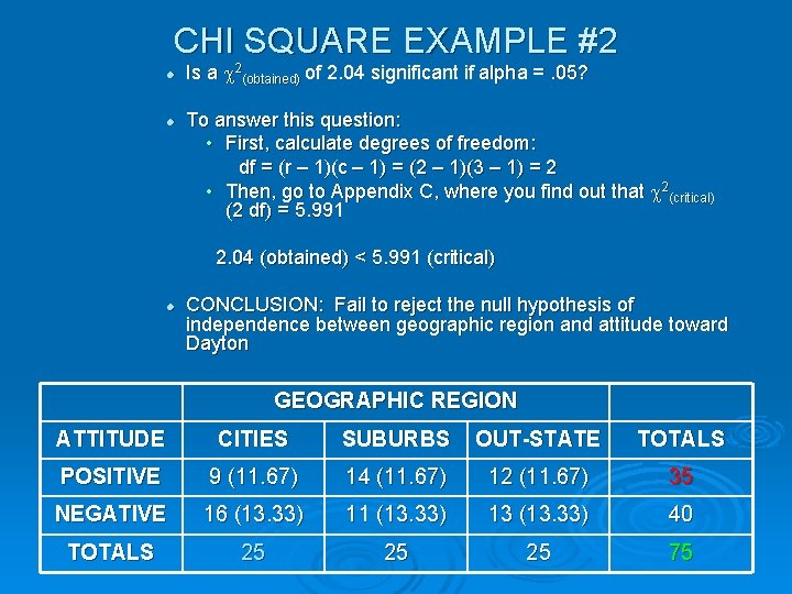
CHI SQUARE EXAMPLE #2 l l Is a 2(obtained) of 2. 04 significant if alpha =. 05? To answer this question: • First, calculate degrees of freedom: df = (r – 1)(c – 1) = (2 – 1)(3 – 1) = 2 • Then, go to Appendix C, where you find out that 2(critical) (2 df) = 5. 991 2. 04 (obtained) < 5. 991 (critical) l CONCLUSION: Fail to reject the null hypothesis of independence between geographic region and attitude toward Dayton GEOGRAPHIC REGION ATTITUDE CITIES SUBURBS OUT-STATE TOTALS POSITIVE 9 (11. 67) 14 (11. 67) 12 (11. 67) 35 NEGATIVE 16 (13. 33) 11 (13. 33) 13 (13. 33) 40 TOTALS 25 25 25 75

Conclusions Ø In the sample, those in the suburbs (56%) were more likely to hold positive attitudes towards Governor Dayton than those from the twin cities (36%) or those from out state (48%). l l However, none of these differences were statistically significant. We cannot conclude that support for the governor varies across regions in Minnesota. What could we change to make these percentages “statistically significant? ”

SPSS Procedure Ø Analyze Descriptive Statistics Crosstabs Rows = DV Ø Columns = IV Ø Cells Ø l Column Percentages Ø Statistics l Chi square

SPSS Exercise Ø Examine the relationship between sex (male/female) and another variable in the GSS data. l l Sex should be the IV (most things cannot change your sex). Is there a relationship in the sample? • Percentages l Is this relationship significant? • Chi square