Contextual Analysis Understanding and Interpreting Multilevel Statistical Models

Contextual Analysis: Understanding and Interpreting Multilevel Statistical Models Jay S. Kaufman, Ph. D University of North Carolina at Chapel Hill June 2007 1

objectives viewers should gain familiarity with: • common terminology for multilevel models • the need to account for clustered data • potential advantage of a biased estimator • the idea of a “shrinkage” estimator • specification of random effects • interpreting the different types of multilevel models 2

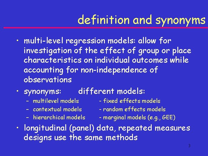
definition and synonyms • multi-level regression models: allow for investigation of the effect of group or place characteristics on individual outcomes while accounting for non-independence of observations • synonyms: different models: – multilevel models – contextual models – hierarchical models - fixed effects models - random effects models - marginal models (e. g. , GEE) • longitudinal (panel) data, repeated measures designs use the same methods 3

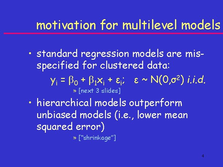
motivation for multilevel models • standard regression models are misspecified for clustered data: yi = 0 + 1 xi + εi; ε ~ N(0, σ2) i. i. d. » [next 3 slides] • hierarchical models outperform unbiased models (i. e. , lower mean squared error) » [“shrinkage”] 4

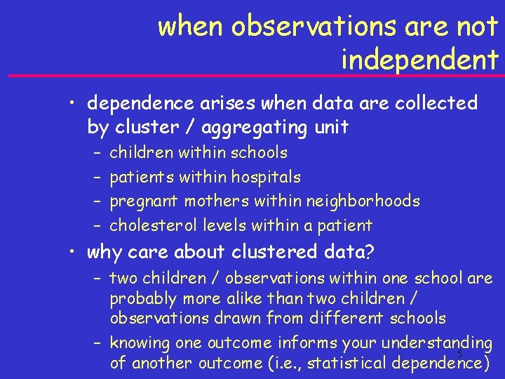
when observations are not independent • dependence arises when data are collected by cluster / aggregating unit – – children within schools patients within hospitals pregnant mothers within neighborhoods cholesterol levels within a patient • why care about clustered data? – two children / observations within one school are probably more alike than two children / observations drawn from different schools – knowing one outcome informs your understanding 5 of another outcome (i. e. , statistical dependence)

when you need multilevel models • reality 1: anytime you have data collected from some aggregate unit / clusters, you will have to use ml models • reality 2: calculating an intraclass correlation coefficient will quantify your clustering (in absence of running a ml model) • reality 3: even if your ‘clustered data’ aren’t empirically clustered, article and grant reviewers may demand it 6

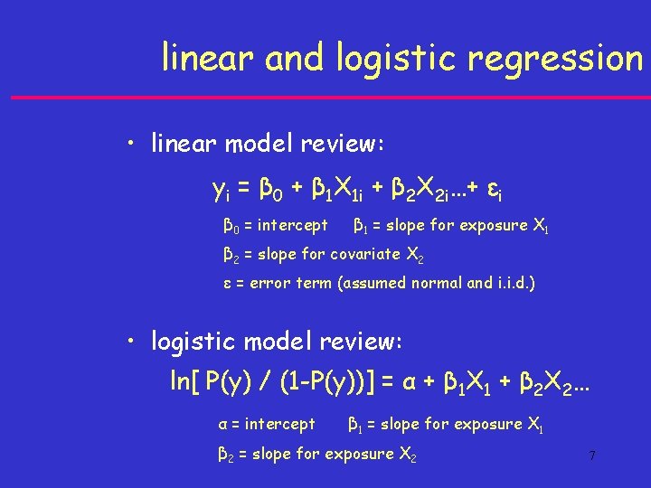
linear and logistic regression • linear model review: yi = β 0 + β 1 X 1 i + β 2 X 2 i…+ εi β 0 = intercept β 1 = slope for exposure X 1 β 2 = slope for covariate X 2 ε = error term (assumed normal and i. i. d. ) • logistic model review: ln[ P(y) / (1 -P(y))] = α + β 1 X 1 + β 2 X 2… α = intercept β 1 = slope for exposure X 1 β 2 = slope for exposure X 2 7

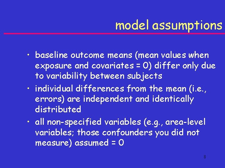
model assumptions • baseline outcome means (mean values when exposure and covariates = 0) differ only due to variability between subjects • individual differences from the mean (i. e. , errors) are independent and identically distributed • all non-specified variables (e. g. , area-level variables; those confounders you did not measure) assumed = 0 8

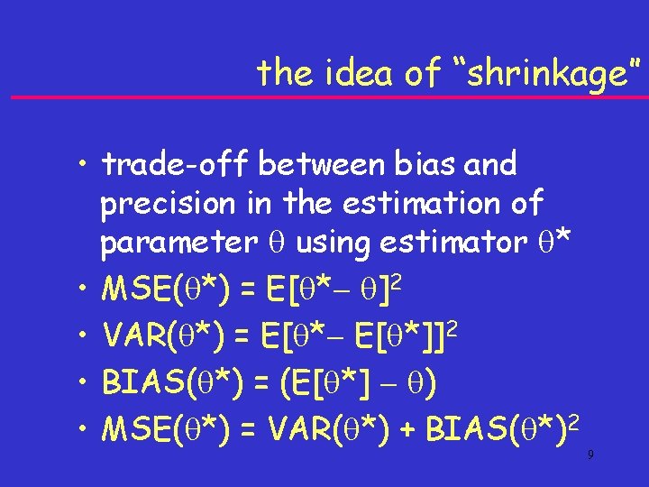
the idea of “shrinkage” • trade-off between bias and precision in the estimation of parameter using estimator * • MSE( *) = E[ * ]2 • VAR( *) = E[ *]]2 • BIAS( *) = (E[ *] ) • MSE( *) = VAR( *) + BIAS( *)2 9

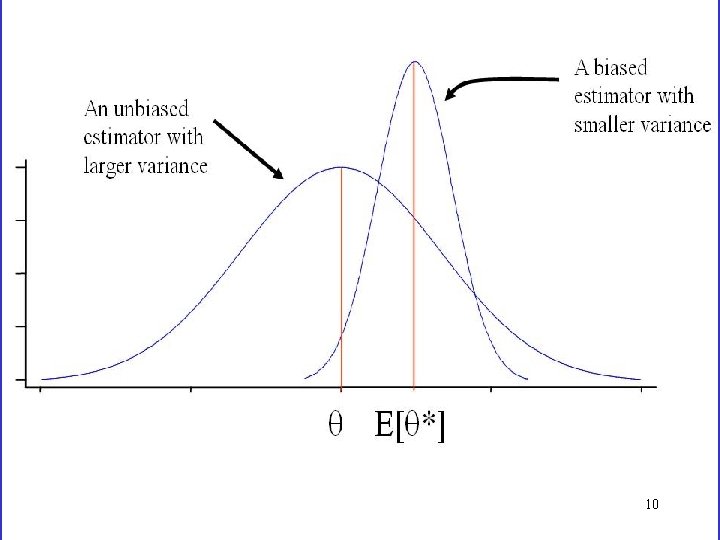
Graphical Depiction of the idea of “shrinkage” 10

efron & morris 1977 [1] Problem: predicting future batting performance of baseball players based on past performance, when there are 3 or more players. Data on 18 major-league players after their first 45 times at bat in the 1970 season. What is known: Player 1: # hits / first 45 times at bat Player 18: # hits / first 45 times at bat To be predicted: Proportion of hits at end of season 11

efron & morris 1977 [2] For each player i, the unbiased estimate of the proportion of hits at end of season is simply the observed proportion of hits out of the first 45: unbiased estimate of i = (# hits / first 45 times at bat for player i) Intuition about regression to the mean : 1) player performances fluctuate at random around their own individual means, and 2) players who have done well in the first 45 times at bat are more likely to have done better than 12 their own player-specific means during this period.

efron & morris 1977 [3] If you had to bet, you'd wager that the worst performing players would do a bit better in the long run and the best players would do a little bit worse in the long run. WHY? Because the player-specific means are more narrowly distributed than the means of the first 45 times at bat, since these estimates include the random sampling variability of each player around his own mean in addition to the natural variation of the player-specific means. 13

efron & morris 1977 [4] 14

the estimation problem [1] Consider estimation of the average risk of preterm delivery among women enrolled in a cohort study. Denote this average risk by (target parameter). Data: observation of A preterm deliveries in a cohort of N enrolled women. Observed proportion (A/N) is the usual estimator of the risk parameter under standard validity assumptions (maximum-likelihood estimator, MLE). 15

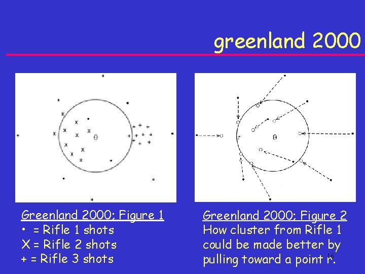
greenland 2000 Greenland 2000; Figure 1 • = Rifle 1 shots X = Rifle 2 shots + = Rifle 3 shots Greenland 2000; Figure 2 How cluster from Rifle 1 could be made better by pulling toward a point 16 r.

the estimation problem [2] In Figure 2, the usual estimator A/N is “shrunk” toward the point r. A Bayesian estimator is an example of a "shrinkage estimator" because it combines prior information with the data. For example, for prior guess r, weight the observed proportion A/N and prior guess r by their sample sizes N and n. Define weight w = N/(N + n), then this estimator is the weighted average: Θb* = w(A/N) + (1 -w)r 17

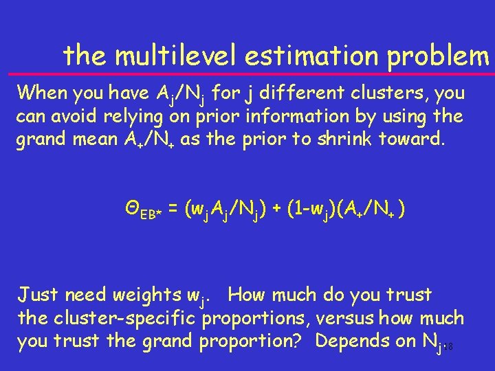
the multilevel estimation problem When you have Aj/Nj for j different clusters, you can avoid relying on prior information by using the grand mean A+/N+ as the prior to shrink toward. ΘEB* = (wj. Aj/Nj) + (1 -wj)(A+/N+ ) Just need weights wj. How much do you trust the cluster-specific proportions, versus how much you trust the grand proportion? Depends on Nj. 18

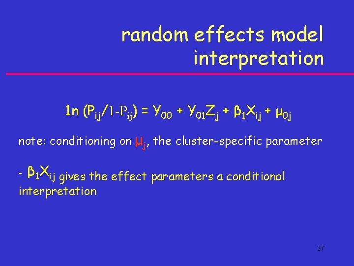
a logistic random intercept models of preterm delivery [1] The simplest hierarchical logistic model expresses the tract-level intercepts 0 j as a function of an overall intercept 00 and tract-specific random deviation terms 0 j. For probability of preterm delivery pij = Pr(yij = 1) for individuals i in tracts j: 1 n (Pij/1 -Pij) = 0 j 0 j = Y 00 + μ 0 j, μ 0 j~ N(0, τ00) 19

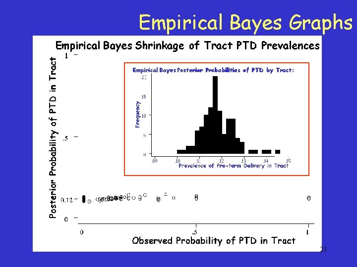
a logistic random intercept models of preterm delivery [2] 00 is the mean of the distribution of random coefficients, estimated as the weighted average of tract intercepts. So both the log-odds of outcome in each tract and 00 (the weighted average of tract-specific log-odds) are estimates for the true tract-specific log-odds. An optimal (minimum MSE) estimator for 0 j is formed by taking the weighted average of these two quantities, with intra-class correlations for weights: 0 j* = λj(β 0 j) + (1 -λj) Ŷ 00 20

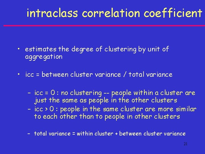
intraclass correlation coefficient • estimates the degree of clustering by unit of aggregation • icc = between cluster variance / total variance – icc = 0 : no clustering -- people within a cluster are just the same as people in the other clusters – icc > 0 : people in the same cluster are more similar to each other than to people in other clusters – total variance = within cluster + between cluster variance 21

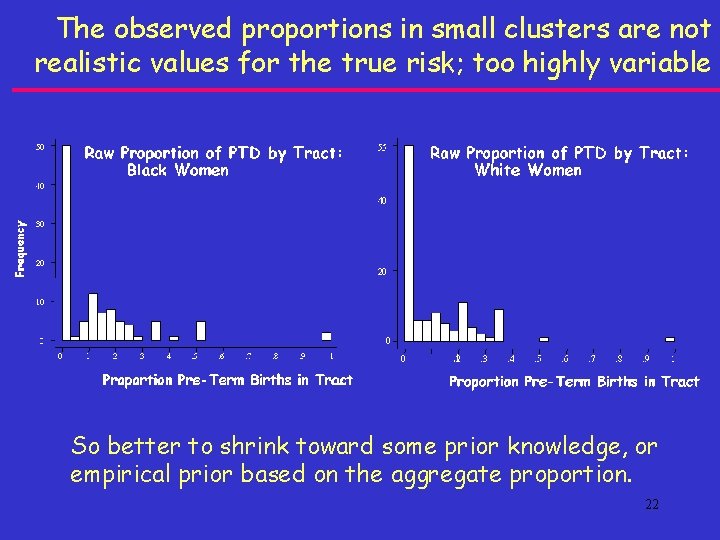
The observed proportions in small clusters are not realistic values for the true risk; too highly variable So better to shrink toward some prior knowledge, or empirical prior based on the aggregate proportion. 22

Empirical Bayes Graphs 23

a logistic random intercept models of preterm delivery [2] Add individual-level or neighborhood-level covariates to explain some of the between tracts variance. For probability of preterm delivery pij = Pr(yij = 1) for individuals i in tracts j: 1 n (Pij/1 -Pij) = 0 j + 1 Xij 0 j = Y 00 + Y 01 Zj + μ 0 j, μ 0 j ~ N(0, τ00) 24

a logistic random intercept models of preterm delivery [3] Replacing the second-level equation into the first level equation yields the combined equation: 1 n (Pij/1 -Pij) = Y 00 + Y 01 Zj + β 1 Xij + μ 0 j These models have random effects only for the intercept, but one could also specify models with random effects for one or more of the slope terms. 25

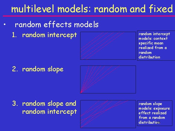
multilevel models: random and fixed • random effects models 1. random intercept models: context specific mean realized from a random distribution 2. random slope 3. random slope and random intercept random slope models: exposure effect realized from a random 26 distribution

random effects model interpretation 1 n (Pij/1 -Pij) = Y 00 + Y 01 Zj + β 1 Xij + μ 0 j note: conditioning on - μj, the cluster-specific parameter β 1 Xij gives the effect parameters a conditional interpretation 27

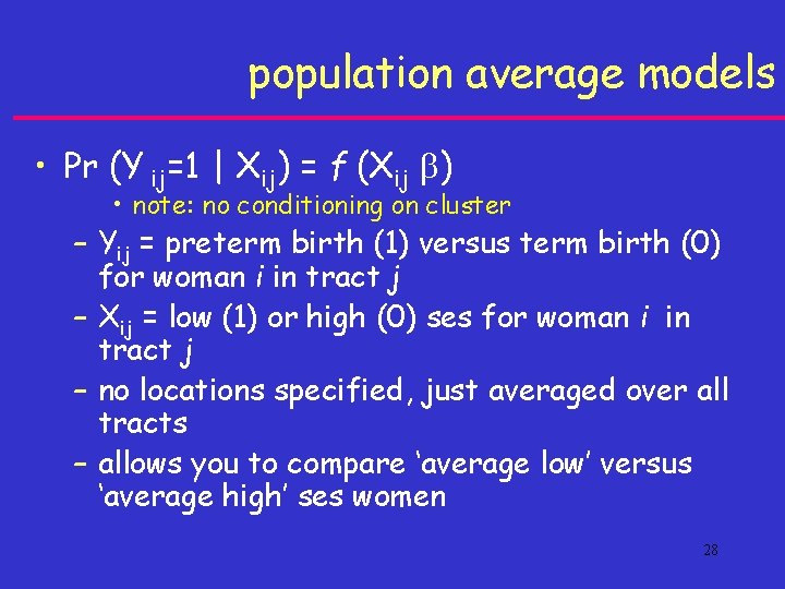
population average models • Pr (Y ij=1 | Xij) = f (Xij ) • note: no conditioning on cluster – Yij = preterm birth (1) versus term birth (0) for woman i in tract j – Xij = low (1) or high (0) ses for woman i in tract j – no locations specified, just averaged over all tracts – allows you to compare ‘average low’ versus ‘average high’ ses women 28

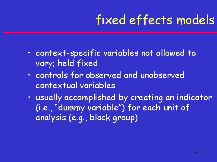
fixed effects models • context-specific variables not allowed to vary; held fixed • controls for observed and unobserved contextual variables • usually accomplished by creating an indicator (i. e. , “dummy variable”) for each unit of analysis (e. g. , block group) 29

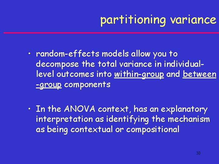
partitioning variance • random-effects models allow you to decompose the total variance in individuallevel outcomes into within-group and between -group components • In the ANOVA context, has an explanatory interpretation as identifying the mechanism as being contextual or compositional 30

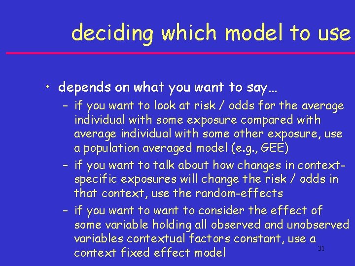
deciding which model to use • depends on what you want to say… – if you want to look at risk / odds for the average individual with some exposure compared with average individual with some other exposure, use a population averaged model (e. g. , GEE) – if you want to talk about how changes in contextspecific exposures will change the risk / odds in that context, use the random-effects – if you want to consider the effect of some variable holding all observed and unobserved variables contextual factors constant, use a 31 context fixed effect model

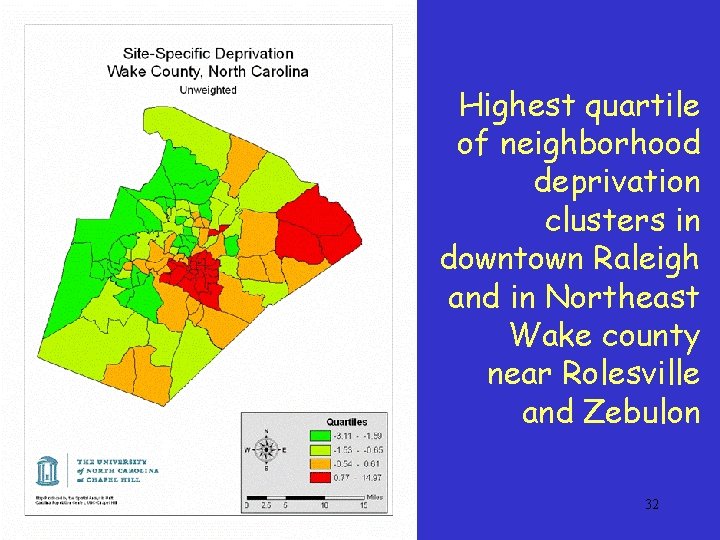
Highest quartile of neighborhood deprivation clusters in downtown Raleigh and in Northeast Wake county near Rolesville and Zebulon 32

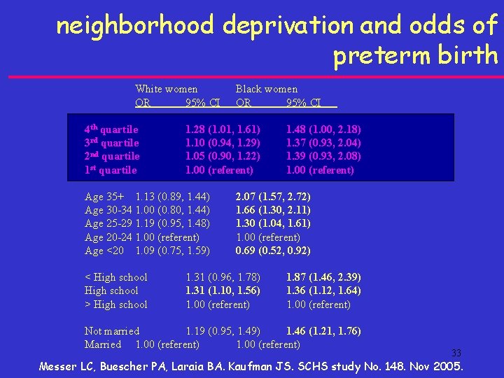
neighborhood deprivation and odds of preterm birth White women OR 95% CI 4 th quartile 3 rd quartile 2 nd quartile 1 st quartile 1. 28 (1. 01, 1. 61) 1. 10 (0. 94, 1. 29) 1. 05 (0. 90, 1. 22) 1. 00 (referent) Age 35+ 1. 13 (0. 89, 1. 44) Age 30 -34 1. 00 (0. 80, 1. 44) Age 25 -29 1. 19 (0. 95, 1. 48) Age 20 -24 1. 00 (referent) Age <20 1. 09 (0. 75, 1. 59) < High school > High school Black women OR 95% CI 1. 48 (1. 00, 2. 18) 1. 37 (0. 93, 2. 04) 1. 39 (0. 93, 2. 08) 1. 00 (referent) 2. 07 (1. 57, 2. 72) 1. 66 (1. 30, 2. 11) 1. 30 (1. 04, 1. 61) 1. 00 (referent) 0. 69 (0. 52, 0. 92) 1. 31 (0. 96, 1. 78) 1. 31 (1. 10, 1. 56) 1. 00 (referent) 1. 87 (1. 46, 2. 39) 1. 36 (1. 12, 1. 64) 1. 00 (referent) Not married 1. 19 (0. 95, 1. 49) 1. 46 (1. 21, 1. 76) Married 1. 00 (referent) 33 Messer LC, Buescher PA, Laraia BA. Kaufman JS. SCHS study No. 148. Nov 2005.

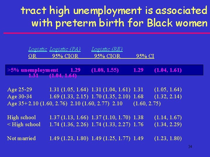
tract high unemployment is associated with preterm birth for Black women Logistic (PA) OR 95% CIOR >5% unemployment 1. 29 1. 31 (1. 04, 1. 64) Logistic (RE) 95% CIOR (1. 08, 1. 55) 95% CI 1. 29 (1. 04, 1. 61) Age 25 -29 1. 31 (1. 05, 1. 64) 1. 31 (1. 04, 1. 61) 1. 31 (1. 05, 1. 64) Age 30 -34 1. 69 (1. 33, 2. 15) 1. 70 (1. 35, 2. 10) 1. 68 (1. 32, 2. 14) Age 35+ 2. 10 (1. 60, 2. 76) 2. 10 (1. 60, 2. 77) 2. 10 (1. 60, 2. 75) High school < High school 1. 37 (1. 13, 1. 66) 1. 37 (1. 10, 1. 70) 1. 38 1. 74 (1. 36, 2. 26) 1. 74 (1. 33, 2. 27) 1. 76 (1. 14, 1. 67) (1. 34, 2. 29) Not married 1. 49 (1. 23, 1. 80) 1. 49 (1. 25, 1. 77) 1. 49 (1. 23, 1. 80) 34

example causal interpretations [1] • population average logistic model (>5% unemployment versus 5% unemployment) OR = 1. 29 (95% CI: 1. 04, 1. 61) the odds of preterm delivery will increase by 29% for a randomly selected woman in a low unemployment if she were to be relocated to a tract with high unemployment 35

example causal interpretations [2] • random effects logistic model (>5% unemployment versus 5% unemployment) OR = 1. 31 (95% CI: 1. 04, 1. 64) the odds of preterm delivery will increase by 31% for a randomly selected woman in a specific census tract with low unemployment if that tract is somehow manipulated to have high unemployment 36

summary • standard regression models assume that data is not clustered by a higher level grouping • one can model clustered data by either using methods robust to this violation of assumptions, or else by modeling this clustering directly • random effects models estimate conditional parameters (i. e. , the effect of exposure given a particular cluster) 37