Contents 1 IC Key process IC IC Packaging

 & Wire bonding")

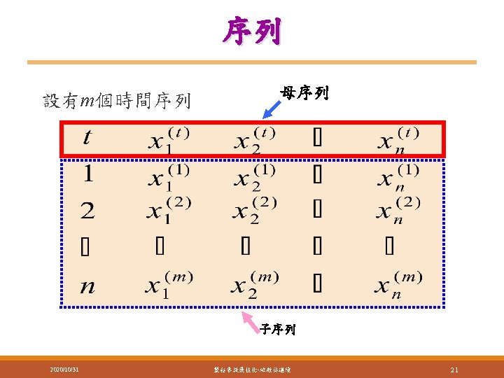
 2.")
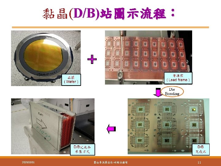
 Wafer (晶圓) Taping (貼研磨膠紙) Wafer Grinding (晶圓研磨站) De-Taping (撕研磨膠紙) Wafer Mount (晶圓貼片) MHD")
 D/B Curing (黏晶烘烤) 3 rd")

 Post Mold Curing (封膠後烘烤) Deject & Trim (沖切去膠站) Visual Check")

 Ø Software: Excel or other packages (Mini. Tab, Jmp,")
 used in an economic design of")


 2020/10/31 製程參數最佳化-離散與連續 40")


1/3 2020/10/31 製程參數最佳化-離散與連續 44")


 EFO (x 2) Bonding power (x")


- Slides: 57
Contents 1. IC封裝測試製程簡介 Ø Key process – IC封裝( IC Packaging ) & Wire bonding 2. Optimization methods Ø Discrete: Taguchi method + Grey relational analysis/FIS Ø Continuous: Neural network, Mathematical modeling Ø Synthetic index: Grey relational analysis/FIS 3. Implementations 2020/10/31 製程參數最佳化-離散與連續 2
PCB assembly 2020/10/31 製程參數最佳化-離散與連續 3
IC Assembly Process Flow l基本 IC 封裝廠流程,可分成三大部份: 1. Pre-Assembly ( 簡稱 P/A ) 2. Assembly-Front End ( 簡稱 F/E ) 3. Assembly-Back End ( 簡稱 B/E ) 晶圓 (Wafer) 成品 (Product) IC封裝 IC測試 功能測試 2020/10/31 製程參數最佳化-離散與連續 4
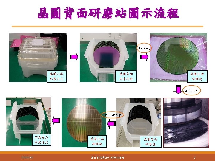
Pre-Assembly(P/A) Wafer (晶圓) Taping (貼研磨膠紙) Wafer Grinding (晶圓研磨站) De-Taping (撕研磨膠紙) Wafer Mount (晶圓貼片) MHD 2020/10/31 2 nd Inspection (第二目檢站) UV (紫外線照射) 製程參數最佳化-離散與連續 Wafer Sawing (晶圓切割站) 5
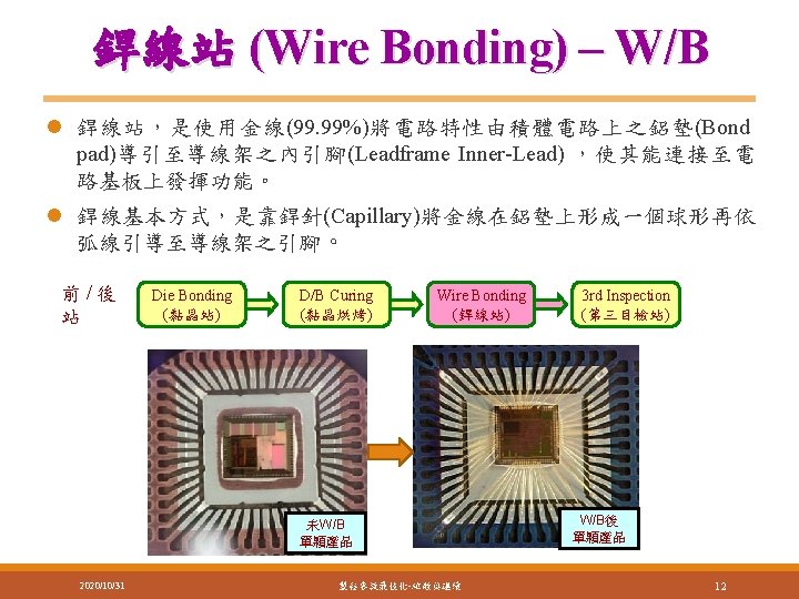
前 段Front-end Process Flow MHD 投料 Die Bonding (黏晶站) D/B Curing (黏晶烘烤) 3 rd Inspection (第三目檢站) Plasma (清洗站) 1 C/C Curing (點膠烘烤) Chip Coating (點膠) 2 Wire Bonding (銲線站) 3 rd Inspection (第三目檢站) 傳送櫃 3 rd Inspection (第三目檢站) 2020/10/31 製程參數最佳化-離散與連續 9
Wire Bonding 2020/10/31 製程參數最佳化-離散與連續 13
後段Back-end 傳送櫃 Molding (封膠站) Post Mold Curing (封膠後烘烤) Deject & Trim (沖切去膠站) Visual Check (外觀檢查站) Form & Singluation (彎腳成型站) TOP Marking (蓋印站) Plating (電鍍站) 2 4 th Inspection (第四目檢站) INK Marking (油墨蓋印) Packing (包裝站) Marking Curing (油墨蓋印後烘烤) 2020/10/31 製程參數最佳化-離散與連續 1 Laser Marking (雷射蓋印) 14
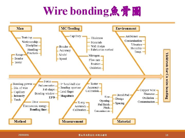
Wire bonding -Mechanics tests 2020/10/31 製程參數最佳化-離散與連續 15
應用方法 1. 田口實驗矩陣(Taguchi Orthogonal array) Ø Software: Excel or other packages (Mini. Tab, Jmp, Design-expert). 2. 類神經網路(Artificial neural network, ANN) Ø Software: Neural. Power, Neuralsolutions… 3. 反應曲面法(Response surface methodology) Ø Software: Design-expert or Mini. Tab 4. 需求轉換函數(Desirability function approach) 2020/10/31 製程參數最佳化-離散與連續 17
田口方法 u The orthogonal arrays and sign-to-noise (S/N) used in an economic design of experiment (DOE) and the Taguchi robust parameter design u S/N ratios based on quality loss function: (1) the smaller-thebetter (STB); (2) the larger-the-better (LTB); and (3) the nominal-the-better (NTB). 2020/10/31 製程參數最佳化-離散與連續 18
Continuous parameter optimization
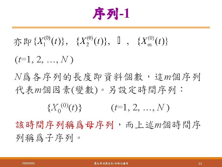
Grey relational analysis Suppose there are m experimental results obtained from an experimental design and n quality characteristics of concern. The data series X 1, …, Xi, …, Xm illustrates the elements of the experimental data in the grey analysis: where Xi denotes the ith experimental results and acts as a comparative sequence in the analysis; k=1, 2, …, n. 2020/10/31 製程參數最佳化-離散與連續 30
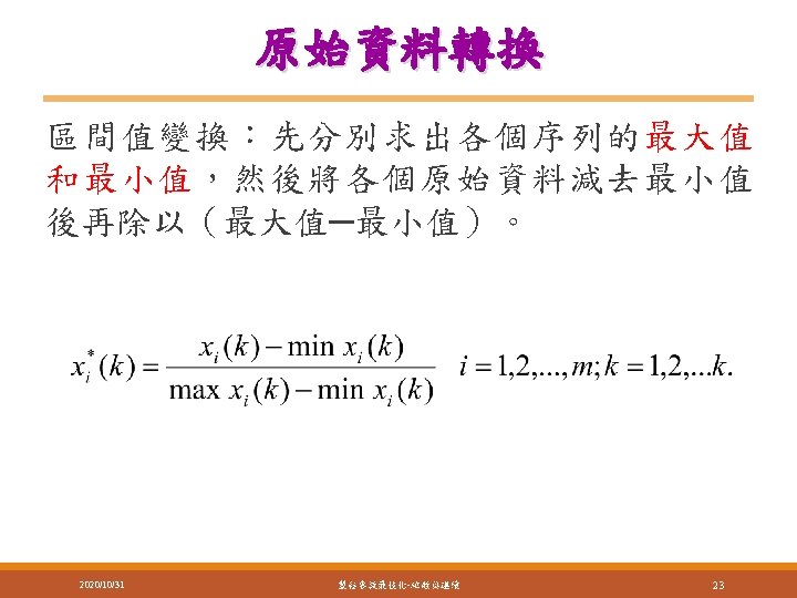
GRA Procedure l Step 1: Normalization: a data sequence may have different range and units. Grey relation generation is performed through a linear transformation to confine the original data sequence within the interval [0, 1]. l The attribute of “larger-the-better” is utilized due to the higher desirability which is preferred for this optimization problem l is the normalized value of the kth element in the ith comparative sequence. 2020/10/31 製程參數最佳化-離散與連續 31
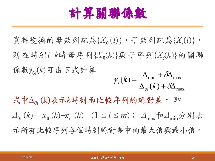
GRA Procedure l Step 2: Calculate the grey relational coefficient: a grey relational coefficient (GRC) is calculated to represent the correlation between the ideal value, x 0(k) and the normalized value. The ideal value is generally set at 1. The GRC for each element, γi(k), can be derived: where γi(k) is the relative difference in the kth element between xi and x 0 in the comparative sequence; ∆oi(k) = ||xo(k)-xi(k)||; ∆min is the minimum value of ∆oi; ∆max is the maximum value of ∆oi; and δ is the distinguishing coefficient which is generally set at 0. 5 2020/10/31 製程參數最佳化-離散與連續 32
GRA Procedure l Step 3: Compute the grey relational grade: A grey relational grade (GRG) is computed to show the degree of similarity between the ith reference sequence and the comparative sequence, by averaging the GRCs using where n is the number of elements. 2020/10/31 製程參數最佳化-離散與連續 33
GRA Procedure l Step 4: Rank the GRG: the GRG shows the desirability of each experimental run. The higher the GRG is, the greater is the desirability. 2020/10/31 製程參數最佳化-離散與連續 34
Optimization methods 2020/10/31 製程參數最佳化-離散與連續 35
DOE – Taguchi 21× 37 Exp. run #1 #2 #3 #4 #5 #6 #7 #8 #9 #10 #11 #12 #13 #14 #15 #16 #17 #18 2020/10/31 Control factors Responses x 1 x 2 x 3 x 4 Wire pull (y 1) 1 1 1 1 1 2 2 2 2 2 1 1 1 2 2 2 3 3 3 1 2 3 1 2 3 2 3 1 3 1 2 製程參數最佳化-離散與連續 7. 78 7. 89 7. 99 7. 68 7. 63 8. 23 7. 35 7. 34 7. 54 7. 45 7. 67 8. 01 7. 81 7. 67 7. 61 8. 10 Ball shear (y 2) 17. 74 21. 32 19. 00 21. 10 21. 68 22. 10 17. 66 20. 60 21. 80 21. 66 21. 30 20. 93 22. 67 21. 20 20. 67 21. 20 21. 66 21. 30 Ball thickness (y 3) 8. 80 8. 90 10. 00 10. 10 10. 20 10. 00 9. 60 10. 80 9. 30 10. 40 9. 80 10. 20 9. 80 9. 50 10. 40 10. 10 10. 50 36
Normal Plot 2020/10/31 製程參數最佳化-離散與連續 37
Grey relational analysis and ranking C 1 Exp. run #1 #2 #3 #4 #5 #6 #7 #8 #9 #10 #11 #12 #13 #14 #15 #16 #17 #18 C 2 C 3 C 4 C 5 C 6 Normalized GRC -Wire pull -Ball shear -Ball Thk. -Wire pull -Ball shear 2020/10/31 0. 49 0. 62 0. 73 0. 38 0. 33 1. 00 0. 01 0. 00 0. 22 0. 11 0. 12 0. 37 0. 75 0. 53 0. 37 0. 30 0. 87 0. 85 0. 02 0. 73 0. 27 0. 69 0. 80 0. 89 0. 00 0. 59 0. 83 0. 80 0. 73 0. 65 1. 00 0. 71 0. 60 0. 71 0. 80 0. 73 0. 00 0. 08 1. 00 0. 92 0. 83 1. 00 0. 67 0. 33 0. 42 0. 67 0. 50 0. 83 0. 58 0. 67 0. 92 0. 58 0. 50 0. 57 0. 65 0. 43 1. 00 0. 34 0. 33 0. 39 0. 36 0. 44 0. 67 0. 51 0. 44 0. 42 0. 79 0. 77 製程參數最佳化-離散與連續 0. 34 0. 65 0. 41 0. 61 0. 72 0. 81 0. 33 0. 55 0. 74 0. 71 0. 65 0. 59 1. 00 0. 63 0. 56 0. 63 0. 71 0. 65 C 7 GRC -Ball Thk. 0. 33 0. 35 1. 00 0. 86 0. 75 1. 00 0. 60 0. 43 0. 46 0. 60 0. 50 0. 75 0. 55 0. 60 0. 86 0. 55 C 8 Weighted GRG 0. 389 0. 523 0. 684 0. 640 0. 632 0. 938 0. 423 0. 437 0. 533 0. 559 0. 504 0. 595 0. 807 0. 632 0. 515 0. 550 0. 786 0. 655 C 9 Rank 18 13 4 6 8 1 17 16 12 10 15 9 2 7 14 11 3 5 38
ANN modeling l Step 5: Nonlinear modeling of the Cu wire bonding process using ANN l The Levenberg-Marquardt (LM) algorithm is proposed with the Sigmoid transfer function to map the nonlinear behavior of the Cu wire bonding process. The processing elements of the neural network are fully connected with one hidden layer. 2020/10/31 製程參數最佳化-離散與連續 39
Response contour of the GRG (Desirability) 2020/10/31 製程參數最佳化-離散與連續 40
GA search Begin GA Initialize a population of 50 elements as a potential solution to prevent premature convergence Evaluate initial population Do while termination criteria are not satisfied Evaluate each individual's fitness by applying the trained LM neural network Select parents for reproduction (Apply evolutionary operators to generate new offspring) Apply crossover operator (Pc=0. 7) Apply mutation operator (Pm=0. 2) Evaluate solutions in the population Check for termination criteria Loop End GA The optimum parameter settings to achieve maximum desirability are determined: the bonding time is set at 11. 9 (Ms), the EFO time is 226. 1 (μs), the bonding power is 110 (US), and the bonding force 6. 5 (gm). 2020/10/31 製程參數最佳化-離散與連續 41
RSM optimization l A quadratic polynomial is normally utilized to approximate a true response surface of a system. Eq is a general form of the approximation function used to formulate the response: where β 0 is a constant; βi is the linear term coefficient; βii stands for the quadratic term coefficient; βi∙j denotes the interaction term coefficient; and denotes a random error component. 2020/10/31 製程參數最佳化-離散與連續 42
RSM optimization l To deal with the multi-objective problem, RSM is usually engaged with the DFA (Derringer and Suich, 1980) to interfuse multiple quality characteristics into an optimization of the overall desirability. Responses Wire pull (y 1) Ball shear (y 2) Ball thickness (y 3) 2020/10/31 Specifications ≥ 3. 5 gm ≥ 11 gm 10± 3 μm 製程參數最佳化-離散與連續 43
RSM optimization D=(d 1 d 2 d 3)1/3 2020/10/31 製程參數最佳化-離散與連續 44
RSM optimization Exp. run #1 #2 #3 #4 #5 #6 #7 #8 #9 #10 #11 #12 #13 #14 #15 #16 #17 #18 2020/10/31 Wire pull (d 1) 0. 956 0. 978 0. 998 0. 936 0. 926 0. 966 0. 870 0. 908 0. 888 0. 890 0. 934 0. 952 0. 962 0. 934 0. 922 0. 964 1. 000 Ball shear (d 2) 0. 749 1. 000 0. 846 1. 000 0. 743 0. 969 1. 000 0. 995 1. 000 0. 975 1. 000 Ball thickness (d 3) 0. 600 0. 633 1. 000 0. 967 0. 933 1. 000 0. 867 0. 733 0. 767 0. 800 0. 933 0. 867 0. 967 0. 833 製程參數最佳化-離散與連續 Overall desirability (D) 0. 755 0. 852 0. 945 0. 967 0. 953 0. 989 0. 824 0. 864 0. 886 0. 916 0. 893 0. 954 0. 961 0. 965 0. 912 0. 928 0. 977 0. 941 Rank 18 16 8 3 7 1 17 15 14 11 13 6 5 4 12 10 2 9 45
RSM optimization 2020/10/31 製程參數最佳化-離散與連續 46
ANOVA results for the quadratic meta-model Source Model A-Bond time B-EFO time C-Bond power D-Bond force BD CD D 2 Residual Cor Total 2020/10/31 Sum of Squares 0. 050015 0. 006615 0. 004099 0. 002038 0. 008299 0. 003005 0. 000651 0. 016669 0. 012947 0. 062969 Mean Square 7 0. 00715 1 0. 00661 1 0. 00410 1 0. 00204 1 0. 00830 1 0. 00301 1 0. 00065 1 0. 01667 10 0. 00129 17 df p-value Prob > F 0. 0081 0. 0474 0. 1055 0. 2381 0. 0298 0. 1586 0. 4942 0. 0049 F-value 5. 51981 5. 10845 3. 16720 1. 57447 6. 41205 2. 32134 0. 50334 12. 87808 製程參數最佳化-離散與連續 Significance significant 47
Optimum parameter sets Factors Bonding time (x 1) EFO (x 2) Bonding power (x 3) Bond force (x 4) Desirability (y. D) 2020/10/31 Set #2 13. 87 12. 67 230 227 100 7. 88 1. 00 製程參數最佳化-離散與連續 Set #3 Set #4 Set #5 108 7. 29 13. 04 226 108 7. 26 13. 85 234 110 7. 85 13. 95 224 110 8. 83 1. 00 48
驗證實驗 Defect types Methods Opportunities/30 packages Oxidation Golf-clubbing Cracked heels Bad wedge bond Wire breakage Neck breaking Weld lift Metallization lift off Cratering Sub-total defects Yield rate Sigma level Short term Cpk Original settings RSM-based approach The proposed approach 960 3 3 2 2 2 5 18 98. 13% 3. 58 1. 19 960 1 1 1 2 0 2 1 0 1 8 99. 17% 3. 89 1. 30 960 0 1 1 0 0 1 3 99. 69% 4. 23 1. 41 FAB Image 2020/10/31 1 st bond/Al Splash Image 2 nd Bond Image 製程參數最佳化-離散與連續 49
Discrete parameter optimization
Optimization flow 2020/10/31 製程參數最佳化-離散與連續 51
實驗設計 Exp. run #1 #2 #3 #4 #5 #6 #7 #8 #9 #10 #11 #12 #13 #14 #15 #16 #17 #18 2020/10/31 A 1 1 1 1 1 2 2 2 2 2 Control factors B C D 1 1 2 2 1 3 3 2 1 1 2 2 3 3 3 1 1 1 3 1 2 1 1 3 2 2 1 2 2 2 3 1 3 3 2 Mean Wire pull ( ) 17. 81 17. 35 17. 23 17. 65 17. 90 17. 86 17. 94 17. 41 17. 89 17. 37 17. 00 17. 68 17. 79 17. 84 17. 67 17. 61 17. 83 17. 71 17. 64 Responses-S/N ratios (db) Ball shear ( ) Ball height( ) 24. 97 16. 59 27. 60 25. 23 25. 09 21. 72 24. 13 20. 00 28. 59 21. 31 28. 29 23. 01 27. 56 25. 73 25. 07 19. 88 28. 61 25. 57 29. 12 25. 57 24. 76 18. 32 26. 41 21. 37 27. 47 25. 57 25. 35 26. 81 28. 36 23. 01 25. 64 21. 37 28. 32 23. 01 25. 32 27. 66 26. 70 22. 87 製程參數最佳化-離散與連續 52
Taguchi method-optimization Responses Factors A: EFO B: Bonding time C: Bonding power D: Bonding force Optimum factor combination 2020/10/31 Wire pull Ball thickness 1 2 Ball shear Optimum factor level 2 2 3 2 A 1 B 2 C 1 D 2 A 2 B 2 C 3 D 2 A 2 B 3 C 3 D 2 製程參數最佳化-離散與連續 2 3 3 2 53
GRA vs. FIS Exp. run #1 #2 #3 #4 #5 #6 #7 #8 #9 #10 #11 #12 #13 #14 #15 #16 #17 #18 GRG -GRA 0. 497 0. 587 0. 421 0. 457 0. 737 0. 716 0. 786 0. 422 0. 820 0. 726 0. 356 0. 530 0. 695 0. 697 0. 648 0. 491 0. 704 0. 689 2020/10/31 Rank 13 11 17 15 3 5 2 16 1 4 18 12 8 7 10 14 6 9 GFG-FIS 0. 541 0. 728 0. 491 0. 494 0. 757 0. 799 0. 500 0. 940 0. 804 0. 378 0. 574 0. 716 0. 761 0. 720 0. 495 0. 808 0. 725 Rank 13 8 17 16 6 7 4 14 1 3 18 12 11 5 10 15 2 9 製程參數最佳化-離散與連續 55
驗證實驗 Parameter Optimal parameter settings Methods Grey-Taguchi method Grey-fuzzy Taguchi method setting used Confirmation PIR Confirmation in mass Improvement Indicators experiment (%) experiment production Factor levels A 1 B 1 C 2 D 2 A 2 B 2 C 3 D 2 --A 1 B 3 C 3 D 2 -Wire pull 17. 35 19. 17 d. B 1. 82 d. B 10. 49 20. 54 d. B 3. 19 d. B S/N ratio Ball shear 27. 60 29. 67 d. B 2. 07 d. B 7. 50 32. 32 d. B 4. 72 d. B S/N ratio Ball height 25. 23 28. 15 d. B 2. 92 d. B 11. 57 30. 17 d. B 4. 94 d. B S/N ratio 2020/10/31 製程參數最佳化-離散與連續 PIR (%) -18. 39 17. 10 19. 58 56
Q&A