Cont Human Gene Mapping Disease Gene Identification MAPPING

Cont. Human Gene Mapping & Disease Gene Identification

MAPPING HUMAN GENES BY LINKAGE ANALYSIS Determining Whether Two Loci Are Linked • Linkage analysis is a method of mapping genes that uses family studies to determine whether two genes show linkage )are linked) when passed on from one generation to the next. • To decide whether two loci are linked, and if so, how close or far apart they are, we rely on two pieces of information. • First, we ascertain whether the recombination fraction between two loci deviates significantly from 0. 5 • Second, if θ is less than 0. 5, we need to make the best estimate we can of θ since that will tell us how close or far apart the linked loci are.

For these determinations, a statistical tool called the likelihood ratio is used. � Likelihoods are probability values; odds are ratios of likelihoods. � One proceeds as follows: � ◦ examine a set of actual family data, count the number of children who show or do not show recombination between the loci, ◦ calculate the likelihood of observing the data at various possible values of θ between 0 and 0. 5. ◦ Calculate a second likelihood based on the null hypothesis that the two loci are unlinked, that is, θ= 0. 50. ◦ take the ratio of the likelihood of observing the family data for various values of θ to the likelihood the loci are unlinked to create an odds ratio.

The computed odds ratios for different values of θ are usually expressed as the log 10 of this ratio and are called a LOD score (Z) for "logarithm of the odds. "

Model-Based Linkage Analysis of Mendelian Diseases � Linkage analysis is called model-based (or parametric) when it assumes that there is a particular mode of inheritance (autosomal dominant, autosomal recessive, or X-linked) that explains the inheritance pattern. � LOD score analysis allows mapping of genes in which mutations cause diseases that follow mendelian inheritance. � The LOD score gives both: a best estimate of the recombination frequency, θmax, between a marker locus and the disease locus; and

� an assessment of how strong the evidence is for linkage at that value of θmax. Values of the LOD score above 3 are considered strong evidence. � Linkage at a particular θ max of a disease gene locus to a marker with known physical location implies that the disease gene locus must be near the marker

The odds ratio is important in two ways. � First, it provides a statistically valid method for using the family data to estimate the recombination frequency between the loci. � If θ max differs from 0. 50, you have evidence of linkage. However, even if θ max is the best estimate you can make, how good an estimate is it? The odds ratio also provides you with an answer to this question because the higher the value of Z, the better an estimate θmax is.

values of Z (odds >1) at a given θ suggest that the two loci are linked, whereas negative values (odds <1) suggest that linkage is less likely than the possibility that the two loci are unlinked. � By convention, a combined LOD score of +3 � Positive or greater (equivalent to greater than 1000: 1 odds in favor of linkage) is considered definitive evidence that two loci are linked.

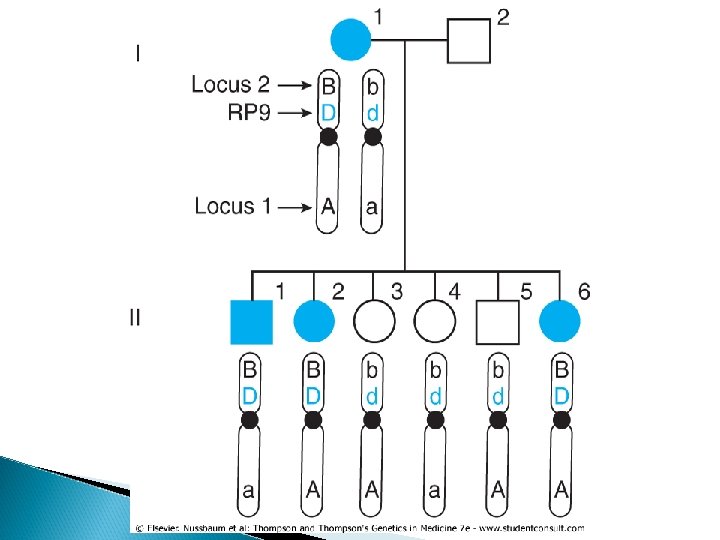
� Mapping genes by linkage analysis provides an opportunity to localize medically relevant genes by following inheritance of the condition and the inheritance of alleles at polymorphic markers to see if the disease locus and the polymorphic marker locus are linked. � Return to the family shown in Figure 10 -6. The mother has an autosomal dominant form of retinitis pigmentosa. She is also heterozygous for two loci on chromosome 7, one at 7 p 14 and one at the distal end of the long arm.

� One can see that transmission of the RP mutant allele (D) invariably "follows" that of allele B at marker locus 2 from the first generation to the second generation in this family. � All three offspring with the disease (who therefore must have inherited their mother's mutant allele D at the RP locus) also inherited the B allele at marker locus 2. All the offspring who inherited their mother's normal allele, d, inherited the b allele and will not develop RP. The gene encoding RP, however, shows no tendency to follow the allele at marker locus 1.

• Suppose we let θ be the "true" recombination fraction between RP and locus 2, the fraction we would see if we had unlimited numbers of offspring to test. • Because either a recombination occurs or it does not, the probability of a recombination, θ, and the probability of no recombination must add up to 1. Therefore, the probability that no recombination will occur is 1 -θ. • There are only six offspring, all of whom show no recombination. Because each meiosis is an independent event, one multiplies the probability of a recombination, θ, or of no recombination, - 1)θ , ( for each child. • The likelihood of seeing zero offspring with a recombination and six offspring with no recombination between RP and marker locus 2 is therefore (θ(0(1 -θ )6. The LOD score between RP and marker 2, then, is: The maximum value of Z is 1. 81, which occurs when θ = 0, and is suggestive of but not definite evidence for linkage because Z is positive but less than 3.

Combining LOD Score Information Across Families � In the same way that each meiosis in a family that produces a nonrecombinant or recombinant offspring is an independent event, so too are the meioses that occur in other families. � We can therefore multiply the likelihoods in the numerators and denominators of each family's likelihood odds ratio together. � An equivalent but more convenient calculation is to add the log 10 of each likelihood ratio, calculated at the various values of θ, to form an overall Z score for all families combined.

� In the case of RP in Figure 10 -6, suppose two other families were studied and one showed no recombination between locus 2 and RP in four children and the third showed no recombination in five children. The individual LOD scores can be generated for each family and added together (Table 10 -1). In this case, one could say that the RP gene in this group of families is linked to locus 2. Because the chromosomal location of polymorphic locus 2 was known to be at 7 p 14, the RP in this family can be mapped to the region around 7 p 14, which is near RP 9, an already identified locus for one form of autosomal dominant RP.

Table 10 -1. LOD Score Table for Three Families with Retinitis Pigmentosa θ 0= θ 0. 01= θ 0. 05= θ 0. 1= θ 0. 2= θ 0. 3= θ 0. 4= Family 1 1. 8 1. 78 1. 67 1. 53 1. 22 0. 88 0. 48 Family 2 1. 19 1. 11 1. 02 0. 82 0. 58 0. 32 Family 3 1. 5 1. 48 1. 39 1. 28 1. 02 0. 73 0. 39 Total 4. 5 4. 45 4. 17 2. 83 3. 06 2. 19 1. 19 Zmax = 4. 5 at θ max = 0

� If, however, some of the families being used for the study have RP due to mutations at another locus, the LOD scores between families will diverge, with some showing a trend to being positive at small values of θ and others showing strongly negative LOD scores at these values. � One can still add the Z scores together, but the result will show a sharp decline in the overall LOD score. � Thus, in linkage analysis involving more than one family, unsuspected locus heterogeneity can obscure what may be real evidence for linkage in a subset of families.

� Phase information is important in linkage analysis. Figure 10 -14 shows two pedigrees of autosomal dominant neurofibromatosis, type 1 (NF 1. ( � In the three-generation family on the left, the affected mother, II-2, is heterozygous at both the NF 1 locus (D/d) and a marker locus (M/m), but we have no genotype information on her parents. � Her unaffected husband, II-1, is homozygous both for the normal allele d at the NF 1 locus and happens to be homozygous for allele M at the marker locus. He can only transmit to his offspring a chromosome that has the normal allele (d) and the M allele.

� By inspection, then, we can infer which alleles in each child have come from the mother. The two affected children received the m alleles along with the D disease allele, and the one unaffected has received the M allele along with the normal d allele. � Without knowing the phase of these alleles in the mother, either all three offspring are recombinants or all three are nonrecombinants.

Figure 10 -14 Two pedigrees of autosomal dominant neurofibromatosis, type 1) NF 1). A, Phase of the disease allele D and marker alleles M and m in individual II-2 is unknown. B, Availability of genotype information for generation I allows a determination that the disease allele D and marker allele M are in coupling in individual II-2. NR, nonrecombinant; R, recombinant.

• Which of these two possibilities is correct? There is no way to know for certain, and thus we must compare the likelihoods of the two possible results. • Given that II-2 is an M/m heterozygote, we assume the correct phase on her two chromosomes is D-m and d-M half of the time and D-M and d-m the other half. • If the phase of the disease allele is D-m , all three children have inherited a chromosome in which no recombination occurred between NF 1 and the marker locus. If the probability of recombination between NF 1 and the marker is θ, the probability of no recombination is - 1)θ , (and the likelihood of having zero recombinant and three nonrecombinant chromosomes is θ 0 (1 -θ)3.

� The contribution to the total likelihood, assuming this phase is correct half the time, is 1/2 θ 0 (1 -θ)3. The other half of the time, however, the correct phase is D -M and d-m, which makes each of these three children recombinants ; the likelihood, assuming this phase is correct half the time, is 1/2 θ 3(1 -θ)0. � To calculate the overall likelihood of this pedigree, we add the likelihood calculated assuming one phase in the mother is correct to the likelihood calculated assuming the other phase is correct. Therefore, the overall likelihood = 1/2(1 -θ)3 + 1/2 (θ 3)/1/8

• By evaluating the relative odds for values of θ from 0 to 0. 5, the maximum value of the LOD score, Zmax , is found to be log(4) = 0. 602 (when θ (0. 0 = Table 10 -2. Because this is far short of a LOD score greater than 3, we would need at least five equivalent families to establish linkage )at θ (0. 0 = between this marker locus and NF 1. • With slightly more complex calculations (made much easier by computer programs written to facilitate linkage analysis), one can calculate the LOD scores for other values of θ )see Table 10 -2. (

Why are the two phases in individual II-2 in the pedigree shown in Figure 10 -14 A equally likely? � First, unless the marker locus and NF 1 are so close together as to produce linkage disequilibrium between alleles at these loci, we would expect them to be in linkage equilibrium. � Second, new mutations represent a substantial fraction of all the alleles in an autosomal dominant disease with reduced fitness, such as NF 1. If new mutations are occurring independently and repeatedly, the alleles that happened to be present at the neighboring linked loci when each mutation occurred in the NF 1 gene will then be the alleles in coupling with the new disease mutation. A group of unrelated families are likely to have many different mutant alleles, each of which is as likely to be in coupling with one polymorphic marker allele at a linked locus as with any other.

� Suppose now that additional genotype information, shown in Figure 10 -14 B, becomes available in the family in Figure 1014 A. By inspection, it is now clear that the maternal grandfather, I-1, must have transmitted both the NF 1 allele (D) and the M allele to his daughter. � This finding does not require any assumption about whether a crossover occurred in the grandfather's germline; all that matters is that we can be sure the paternally derived chromosome in individual II-2 must have been D-M and the maternally derived chromosome was d-m.

� The availability of genotypes in the first generation makes this a phase-known pedigree. � The three children can now be scored definitively as nonrecombinant and we do not have to consider the opposite phase. � The probability of having three children with the observed genotypes is now (1 -θ )3. As in the previous phase-unknown pedigree, the probability of the observed data if there is no linkage between the loci is (1/2)3 = 1/8. � Overall, the relative odds for this pedigree are (1 θ)3 ÷ 1/8 in favor of linkage, and the maximum LOD score Z at θ= 0. 0 is 0. 903 or 8 to 1 (see Table 10 -2). � Thus, the strength of the evidence supporting linkage (8 to 1) is twice as great in the phaseknown situation as in the phase-unknown situation (4 to 1).

Determining Phase from Pedigrees � As shown in the pedigree in Figure 10 -14 B, having grandparental genotypes may be helpful in establishing phase in the next generation. � However, depending on what the genotypes are, phase may not always be definitively determined. For example, if the grandmother, I-2, had been an M/m heterozygote, it would not be possible to determine the phase in the affected parent, individual II-2.

Determining Phase from Pedigrees � For linkage analysis in X-linked pedigrees, the mother's father's genotype is particularly important because, as illustrated in Figure 10 -15, it provides direct information on linkage phase in the mother. � Because there can be no recombination between Xlinked genes in a male and because the mother always receives her father's only X, any X-linked marker present in her genotype, but not in her father's, must have been inherited from her mother. � Knowledge of phase, so important for genetic counseling, can thus be readily ascertained from the appropriate male members of an X-linked pedigree, if they are available for study.

Pedigree of X-linked hemophilia. The affected grandfather in the first generation has the disease (mutant allele h) and is hemizygous for allele M at an Xlinked locus. No matter how far apart the marker locus and the factor VIII gene are on the X, there is no recombination involving the X-linked portion of the X chromosome in a male, and he will pass the hemophilia mutation h and allele M together. The phase in his daughter must be that h and M are in coupling

MAPPING OF COMPLEX TRAITS � 1. 2. Two major approaches to locate and identify genes that predispose to complex disease or contribute to genetic variance of quantitative traits Affected pedigree member method: if a region of genome is shared more frequently than expected by relatives concordant for a particular disease, the inference is alleles predispose to disease at one or more loci in that region. Association: looks for increased frequency of particular alleles in affected compared with unaffected in the pop.

Model-Free Linkage Analysis of Complex Traits � Linkage analysis is called model-free (or nonparametric) when it does not assume any particular mode of inheritance (autosomal dominant, autosomal recessive, or X-linked) to explain the inheritance pattern.

MAPPING OF COMPLEX TRAITS � Nonparametric LOD (NPL) score analysis allows mapping of genes in which variants contribute to susceptibility for diseases (so-called qualitative traits) or to physiological measurements (known as quantitative traits) that do not follow a straightforward mendelian inheritance pattern.

MAPPING OF COMPLEX TRAITS � NPL scores are based on testing for excessive allelesharing among relatives, such as pairs of siblings, who are both affected with a disease or who show greater similarity to each other for some quantitative trait compared with the average for the population.

MAPPING OF COMPLEX TRAITS � The NPL score gives an assessment of how strong the evidence is for increased allele sharing near polymorphic markers. A value of the NPL score greater than 3. 6 is considered evidence for increased allelesharing; an NPL score greater than 5. 4 is considered strong evidence.

Model-Free Linkage Analysis of Qualitative (Disease) Traits � One type of model-free analysis is the affected sibpair method. � Only siblings concordant for a disease are used � No assumptions need be made about the number of loci involved or the inheritance pattern. � Sibs are analyzed to determine whethere are loci at which affected sibpairs share alleles more frequently than the 50% expected by chance alone � In this method, DNA of affected sibs is systematically analyzed by use of hundreds of polymorphic markers throughout the entire genome in a search for regions that are shared by the two sibs significantly more frequently than is expected on a purely random basis.

� When elevated degrees of allele-sharing are found at a polymorphic marker, it suggests that a locus involved in the disease is located close to the marker. � Whether the degree of allele-sharing diverges significantly from the 50% expected by chance alone can be assessed by use of a maximum likelihood odds ratio to generate a nonparametric LOD score for excessive allele sharing.

Model-Free Linkage Analysis of Quantitative Traits � Model-free linkage methods based on allelesharing can also be used to map loci involved in quantitative complex traits. Although a number of approaches are available, one interesting example is the highly discordant sibpair method. � Once again, no assumptions need be made about the number of loci involved or the inheritance pattern. � Sibpairs with values of a physiological measurement that are at opposite ends of the bell-shaped curve are considered discordant for that quantitative trait and can be assumed to be less likely to share alleles at loci that contribute to the trait.

� The DNA of highly discordant sibs is then systematically analyzed by use of polymorphic markers throughout the entire genome in a search for regions that are shared by the two sibs significantly less frequently than is expected on a purely random basis. � When reduced levels of allele-sharing are found at a polymorphic marker, it suggests that the marker is linked to a locus whose alleles contribute to whatever physiological measurement is under study.

Disease Association � An entirely different approach to identification of the genetic contribution to complex disease relies on finding particular alleles that are associated with the disease. � The presence of a particular allele at a locus at increased or decreased frequency in affected individuals compared with controls is known as a disease association. � In an association study, the frequency of a particular allele (such as for an HLA haplotype or a particular SNP or SNP haplotype) is compared among affected and unaffected individuals in the population

Disease Association patients control total With allele a b a+b Without allele c d c+d total a+c b+d The RRR is approximately equal to the odds ratio when the disease is rare (i. e. , a < b and c < d). (Do not confuse RRR (relative risk ratio) with λr, the risk ratio in relatives. λr is the prevalence of a particular disease phenotype in an affected individual's relatives versus that in the general population. )

If the study design is a case-control study in which individuals with the disease are selected in the population, a matching group of controls without disease are then chosen, and the genotypes of individuals in the two groups are determined; an association between disease and genotype is then calculated by an odds ratio. � Odds are ratios. With use of the above table, the odds of an allele carrier's developing the disease is the number of allele carriers that develop the disease (a) divided by the number of allele carriers who do not develop the disease (b). Similarly, the odds of a noncarrier's developing the disease is the number of noncarriers who develop the disease (c) divided by the number of noncarriers who do not develop the disease (d). The disease odds ratio is then the ratio of these odds, that is, a ratio of ratios. �

� If the study was designed as a cross-sectional or cohort study, in which a random sample of the entire population is chosen and then analyzed both for disease and for the presence of the susceptibility genotype, the strength of an association can be measured by the relative risk ratio (RRR). � The RRR compares the frequency of disease in all those who carry a susceptibility allele ([a/(a + b)] with the frequency of disease in all those who do not carry a susceptibility allele ([c/(c + d)].

� The RRR is approximately equal to the odds ratio when the disease is rare )i. e. , a < b and c < d. ( � The significance of any association can be assessed in one of two ways: ◦ One is simply to ask if the values of a, b, c, and d differ from what would be expected if there were no association by a χ2 test. ◦ The other is determined by a 95% confidence interval for the relative risk ratio. This interval is the range in which one would expect the RRR to fall 95% of the time that you genotype a similar group of cases and controls by chance alone. If the frequency of the allele in question were the same in patients and controls, the RRR would be 1. Therefore, when the 95% confidence interval excludes the value of 1, then the RRR deviates from what would be expected for no association with P value <0. 05.

, Example suppose there were a case-control study in which a group of 120 patients with cerebral vein thrombosis(CVT) Patients with CVT Controls without CVT Total 20210 G > A allele present 23 4 27 20210 G > A allele absent 97 116 213 Total 120 240

� For example, suppose there were a case-control study in which a group of 120 patients with cerebral vein thrombosis (CVT) and 120 matched controls were genotyped for the 20210 G > A allele in the prothrombin gene. � There is clearly a significant increase in the number of patients carrying the 20210 G > A allele versus controls (χ2 = 15 with 1 df; P < 10 -10). Since this is a case-control study, we use an odds ratio (OR) to assess the strength of the association.

Genome-Wide Association and the Haplotype Map � Association studies for human disease genes have been limited to particular sets of variants in restricted sets of genes. For example, geneticists might look for association with variants in genes encoding proteins thought to be involved in a pathophysiological pathway in a disease. � Many such association studies were undertaken before the Human Genome Project era, with use of the HLA loci, because these loci are highly polymorphic and easily genotyped in case-control studies.

Genome-Wide Association and the Haplotype Map � A more powerful approach, however, would be to test systematically for association genome-wide between the more than 10 million variants in the genome and a disease phenotype, without any preconception of what genes and genetic variants might be contributing to the disease. � Although such a massive undertaking is not currently feasible, recent advances in genomics, building on the Hap. Map, make possible an approximation to a full-scale genome-wide association that still retains sufficient power to detect significant associations across the entire genome

Tag SNPs � By examining all the haplotypes within an LD block and measuring the degree of LD between them, it is possible to identify the most useful, minimum set of SNP alleles (so-called tag SNPs) that are capable of defining most of the haplotypes contained in each LD with minimum redundancy. � In theory, a set of well-chosen tag-SNPs constitutes the minimal numbers of SNPs that need to be genotyped to provide nearly complete info on which haplotypes are present on any chromosome

� In practice, genotyping a few hundred thousand tag SNPs is only a bit less useful for an association study than is genotyping more than 10 million SNP genotypes at every known variant in the genome. � Tag SNPs need to be examined and refined before we know if the results based on the four populations studied in the Hap-Map project are applicable world-wide.

From Gene Mapping to Gene Identification � Positional cloning: Mapping location of a disease gene by linkage analysis or other means, followed by identifying the gene on basis of its map position � This strategy has led to identification of genes associated with hundreds of mendelian disorders and to a small but increasing number of genes associated with complex disorders.