Consumption and Investment Unit 3 At the end

Consumption and Investment Unit 3 At the end of this unit, you should be able to: • Define the term consumption, saving and investment • Explain the absolute income hypothesis, recognising the relationship between consumption and saving. • Define the term marginal propensity to consume (and save) and average propensity to consume (and save). • Explain the main features of the permanent income, the life-cycle and the relative income hypotheses as alternatives to the absolute income hypothesis. • Explain the accelerator theory of investment and discuss other possible influences on aggregate investment.

Consumption and Investment • Consumption is the flow of households’ spending o goods and services which yield utility in the current period. • Saving is that part of disposable income which is not spent. • In a closed economy • Yd = C+S • Investment is firms 'spending on goods which are not for current consumption but which yield a flow of consumer goods and services in the future. • The different between consumption spending and total consumption • Consumption spending is the actual amount spent on new consumer goods in the current period. • Total consumption is the using up of consumer goods (both those purchased in the current period and those purchased in past periods which are still providing services to the household)

The absolute income hypothesis The Absolute Income Hypothesis is theory of consumption proposed by English economist John Maynard Keynes The absolute income hypothesis state that consumption depends on current disposable income • consumption and saving are both directly and linearly related to current disposable income. • Consumption and saving functions of the absolute income hypothesis can be illustrated either numerical, graphically or algebraically.

The absolute income hypothesis Numerical illustration of Consumption and saving functions Disposable Income (N$) Consumption (N$) Saving (N$) 250 210 40 200 170 30 150 130 20 100 90 10 50 50 0 0 10 -10 Do the graphical illustration from the table above

The absolute income hypothesis Average propensity consume is equal total consumption divided by total disposable income and it varies as disposable income varies. C 200 150 100 50 Consumption APC at point A = 50/50 =1 APC at point B = 90/100 = 0. 9 B A 0 50 100 150 200 Disposable income

The absolute income hypothesis Algebraic illustration of consumption and saving functions. Yd=C+S C=a+b. Yd S=Yd-C S=Yd-a-b. Yd S=-a+Yd(1 -b) S=-a+(1 -b)Yd mpc + mps=1 b+(1 -b) = 1 or mpc+mps =1

The absolute income hypothesis Let us use the previous table to construct consumption function and saving function Consumption function C = a+b. Yd b= d. C/d. Yd = mpc b= (170 -210)/(200 -250) b= -40/-50 =0. 8 = mpc 210 = a + 0. 8(250) 210 = a + 200 210 -200 = a 10 = a Therefore consumption function is C = 10 +0. 8 Yd

The absolute income hypothesis Saving function S = x + d. Yd d= ds/d. Yd = mps d= (30 -40)/(200 -250) d =-10/-50 d =0. 2 = mps S=x+0. 2(Yd) 40=x+0. 2(250) 40=x+50 40 -50=x =-10 Therefore saving function is S= -10+0. 2 Yd

The absolute income hypothesis The following points represent the major characteristics of the absolute income hypothesis: 1. Consumption and saving are stable functions of current disposable income. The relationships are positive. 2. The relationships are linear but it is also possible for consumption and saving lines to be curved in such a way that the mpc falls as income rises and the mps rises as income rises 3. The mpc lies between zero and one (0<mpc<1) 4. The apc falls as income rises and is greater than the mpc.

Permanent Income Hypothesis The permanent income hypothesis (PIH) is an economic theory about consumption, first developed by Milton Friedman. Permanent consumption (Cp) is proportional to permanent income (Yp) It state that a person's consumption in a year is determined not just by their income in that year but also by their expected income in future years. Therefore consumption depends on permanent income, which is the present value of expected flow of long term income. In its simplest form, the hypothesis states that changes in permanent income, rather than changes in temporary income, are what drive the changes in a consumer's consumption patterns. Cp = k. Yp where k is constant and equal to the average and marginal propensities to consume.

Permanent Income Hypothesis Permanent income is the present value of the expected flow of income from the existing stock of both human and non-human wealth over a long period of time. Human wealth is the source of income received from the sale of labour service, while non-human wealth is the sources of all other income (that is, incomes received from ownership of all kinds of assets, like government bonds, company stocks and shares, and property). Friedman points out that Current measured income (Y) for a household or for the economy as a whole could be greater or less than permanent income.

Permanent Income Hypothesis The difference between the two is called Transitory income which is the different between current measured income and permanent income. In other word, transitory income can be thought of as a temporary, unexpected rise or fall in income (example , an unexpected increase in income resulting from a win at the races, or a temporary fall in income resulting from a short period of unemployment) Current measured income = Permanent income + Transitory Income Y = Yp + Yt The average transitory income level will be equal to zero, therefore the average permanent income would be just equal to the average measured income. (Yp =Y)

Permanent Income Hypothesis Permanent consumption ( Cp) can be thought of as the normal or planned level of spending out of permanent income and can differ from measured consumption ( C) by any unplanned , temporary increases or decreases in consumer spending, called transitory consumption. C = Cp +Ct Two assumptions about transitory consumption 1. Transitory consumption is not correlated with permanent consumption 2. Transitory consumption is not correlated with transitory income which means temporary increases in income do not cause temporary increases in consumption. On average transitory consumption is equal to zero, therefore measured consumption must be equal to permanent consumption. C = k. Yp

Permanent Income Hypothesis Friedman’s consumption function C C = k. Yp Slope = K = apc=mpc 0 Permanent income The relationship between consumption and permanent income is represented by a straight line through the origin with a slope equal to apc and mpc. Wealth also part of the permanent income.

The life-cycle hypothesis developed by Ando and Modigliani in the 1950 s. The hypothesis claims that each individual household will make an estimate of its expected life-time income and will then devise a long-term consumption plan based on this estimate. – Early years of income earning (say from age 18 to 30), households spend more than their current income. Availability of consumer credit facility can be the driving force. – Middle years of income earning (say, from age 30 to 60), household will spend less than its income, partly to repay earlier debts and partly to accumulate wealth for use in later years. – After retirement, this accumulated wealth is gradually depleted as once again dissaving occurs.

• An individual household’s consumption will not necessarily be constant throughout the household’s life-time. • Instead, in any given year, some households will be spending more than their planned average annual consumption and others will be spending less. • In aggregate, these differences will tend to cancel each other out, so that aggregate longrun consumption will tend to be proportional to some measure of long-run income.

Y Income curve Saving C Y Dissaving 15 25 35 45 55 65 75 Lifetime

Relative income hypothesis • Proposed by J. S. Duesenberry in 1949, states that: • A household’s consumption depends not only on its own income, but also on the income of the other households which it observes. • Households will spend more on consumption if it lives in a neighbourhood in which its income is relatively low than if it lives in a neighbourhood in which its income is relatively high.

Investment • Real investment – the addition to the stock of physical capital. • New expenditure incurred on addition of capital goods such as machines, buildings, equipment, tools etc – All firms have to undertake investment expenditure (new plant, machinery and other equipment must be replaced when wear out, – Firms need to acquire additional capital if they are to grow and remain technologically competitive. – Also firms hold stocks of raw materials and semi-finished goods and finished goods • Firms hold stocks for three main reasons: (a) Raw materials have to be held in sufficient quantities to allow production process to take place smoothly (b) Holding stock enable s firms to meet unexpected increase in demand for final product, (c) Raw materials may be bought and held in stocks if future rises in raw materials are expected

• Investment always involve opportunity cost. • If a firm borrows funds to finance an investment, the opportunity cost is represented by the interest rate that must be paid on the borrowed funds. • If new partners or shareholders are brought in, the opportunity cost is the rate of return that must be offered to make it worth their while.

Type of investment 1. Business investment – investment in machinery, tools and equipment that business use in further production of goods and services. 2. Residential investment – expenditure on constructing or buying new houses or dwelling apartments for purpose of living or renting out to others 3. Inventory investment – inventory of raw materials, semi-finished goods and final goods.

Autonomous investment and Induced investment • Autonomous investment – does not change with the change in the income level and is therefore independent of income. • This investment take place in houses, roads, public undertakings and other types of economic infrastructure such as power, transport and communication. • Autonomous investment depends more on population growth and technical progress than on the level of income.

• Induced investment- depends more on income than on the rate of interest. • Increase in national income lead to increase in induced investment. Induced investment Investment Autonomous investment Id I’a Ia Id 0 National income

Investment and the rate of interest • Classical economists viewed the rate of interest as the main determinant of investment. • Consider the microeconomic analysis of a single profit-maximising firm deciding whether or not to undertake an investment, • When a firm buys a new machine, it expects the yield of the investment to exceed cost.

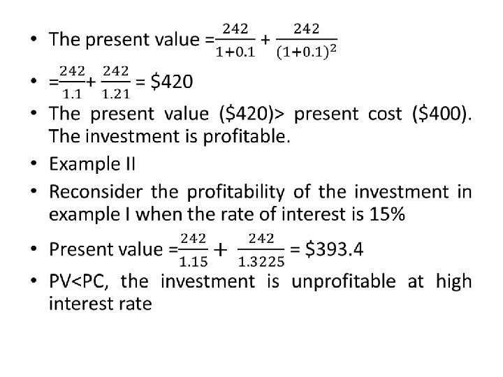
• One way of comparing the expected yield of an investment to its cost is to calculate the present value of the investment and to compare that with the present cost. If present value > present cost, the investment is regarded as profitable. • Example I: suppose a machine which has a known life of only two years is expected to yield $242 each year. The machine present cost is $400 and a rate of interest is 10%. Is the investment profitable?

Calculating the rate of return •

• Example IV • Reconsider the profitability in example III, when the rate of interest is 15% • As calculated in example III, the rate of return from the investment is = 12. 5% • Rate of return 12. 5% < Interest rate, 15%, the investment is unprofitable at high interest rate. – Marginal efficiency of investment (MEI)- the rate of discount which would equate the present value of expected stream of future income from an investment project to the initial outlay. In other words, it is the expected rate of return from an additional dollar of planned investment

• A fall in the market rate of interest should make profitable some investments in the economy which were previously unprofitable, so that aggregate investment should increase. • Similarly, a rise in the market interest rate of interest rate should make unprofitable some investments which where previously profitable, so that aggregate investment should fall. • Therefore aggregate investment is inversely related to the rate of interest

0 Rate of interest I I Investment

The accelerator theory • The view that the level of current net investment depends on past changes in national income. • According to the accelerator theory, the level of current net investment depends on past income, this can be expressed as follows: • It = v(Yt- Yt-1), • Where It = net investment Yt = current national income, Yt-1 =national income in the previous period and v = constant known as accelerator coefficient. • V is also the marginal capital-output ratio

• Gross investment is equal to net investment plus any replacement investment which takes place because of depreciation, written as follows: • GIt = v(Yt – Yt-1)+Rt • Where GIt =current gross investment and Rt = replacement investment. • Replacement investment – the investment necessary to replace obsolete and worn-out equipment • In order for accelerator theory to be valid, firm must demand additional capital to meet any increases in demand for their product

• Calculated example: • income in the t period = 1050, and in t-1=1000 and v=0. 5, what is our investment (I) according to accelerator theory? • Answer: It = 0. 5(1050 -1000) • It =0. 5 (50) = $25 • Use the same example where our replacement investment equal $10 • GIt = 0. 5(1050 -1000)+10 = $25 + $10 =$30

Criticism of accelerator theory 1. It assumes that firms faced with increased demand for their product will immediately attempt to increase their capital stock. This imply that there is no excess capacity ( that all existing machines must be fully employed and there must be no possibility of overtime work or shift work). 2. It fails to take into account business expectations. If businesses regard the increase in demand as temporary, they may not respond to it at all.

Profit as determinant of investment • It is argued that higher levels of profit in the economy will lead to higher level of aggregate investment. This is because higher profits level will increase the availability of funds for investment. • Higher profits may also boost business confidence and so raise the expected future income from planned investment project.

The ‘crowding out’ effect • Finance required by the government to pay for growth of public spending has the effect of raising taxes on incomes and profits, and pushing up interest rate. • This squeezes the profitability of private firms and raises their investment costs • The argument leads to the conclusion that excessive growth in public spending ‘crowds out’ private investment spending.

Overall view of investment •

Time Period Demand Desired stock Net investment (no. of machine Depreciatio n (no of machine Gross investment (No. of machine 0 5000 100 0 1 6000 120 20 10 30 2 10000 200 80 10 90 3 12000 240 40 10 50 4 12000 240 0 10 10 5 10000 200 -40 10 -30