Constraint Satisfaction Problems Chapter 6 1 6 4

Constraint Satisfaction Problems Chapter 6. 1 – 6. 4 Derived from slides by S. Russell and P. Norvig, A. Moore, and R. Khoury

Constraint Satisfaction Problems (CSPs) • Standard search problem: – state is a "black box“ – any data structure that supports successor function, heuristic function, and goal test • CSP: – state is defined by variables Xi with values from domain Di – goal test is a set of constraints specifying allowable combinations of values for subsets of variables – Use a variable-based model • Solution is not a path but an assignment of values for a set of variables that satisfy all constraints

Example: 8 -Queens

Example: Cryptarithmetic • Variables: F, T, U, W, R, O, X 1, X 2 , X 3 • Domains: {0, 1, 2, 3, 4, 5, 6, 7, 8, 9} • Constraints: Alldiff (F, T, U, W, R, O) – O + O = R + 10 · X 1 – X 1 + W = U + 10 · X 2 – X 2 + T = O + 10 · X 3 – X 3 = F, T ≠ 0, F ≠ 0

Example: Movie Seating

Example: Graph Coloring V 3 V 5 V 1 V 2 V 6 V 4 R G • Each circle marked V 1. . V 6 must be assigned R, G or B • No two adjacent circles may be assigned the same color • Note: 2 variables have already been assigned a color in this example

Other Applications of CSPs • Assignment problems – e. g. , who teaches what class • Timetable problems – e. g. , which class is offered when and where? • Scheduling problems • VLSI or PCB layout problems • Boolean satisfiability • N-Queens • Graph coloring • Games: Minesweeper, Magic Squares, Sudoku, Crosswords • Line-drawing labeling Note: many problems require real-valued variables

Example: Map-Coloring Note: In general, 4 colors are necessary • Variables: WA, NT, Q, NSW, V, SA, T • Domains: Di = {red, green, blue} • Constraints: adjacent regions must have different colors e. g. , WA ≠ NT, or (WA, NT) in {(red, green), (red, blue), (green, red), (green, blue), (blue, red), (blue, green)}

Example: Map-Coloring Solutions are complete (i. e. , all variables are assigned values) and consistent (i. e. , does not violate any constraints) assignments, e. g. , WA = red, NT = green, Q = red, NSW = green, V = red, SA = blue, T = green

Constraint Graph • Binary CSP: each constraint relates two variables • Constraint graph: nodes are variables, arcs are constraints

Varieties of CSPs • Discrete variables – finite domains: • n variables, domain size d O(dn) complete assignments • e. g. , Boolean CSPs, Boolean satisfiability – infinite domains: • integers, strings, etc. • e. g. , job scheduling, variables are start/end times for each job • Continuous variables – e. g. , start/end times for Hubble Space Telescope observations

Kinds of Constraints • Unary constraints involve a single variable – e. g. , SA ≠ green • Binary constraints involve pairs of variables – e. g. , SA ≠ WA • Higher-order constraints involve 3 or more variables – e. g. , cryptarithmetic column constraints

Local Search for CSPs • Hill-climbing, simulated annealing, genetic algorithms typically work with "complete" states, i. e. , all variables have values at every step • To apply to CSPs: – allow states with some unsatisfied constraints – operators assign a value to a variable • Variable selection: randomly select any conflicted variable • Value selection by min-conflicts heuristic: – choose value that violates the fewest constraints, i. e. , hill-climb by minimizing f(n) = total number of violated constraints

Local Search Min-Conflicts Algorithm: 0. Assign to each variable a random value, defining the initial state 1. while state not consistent do 2. 1 Pick a variable, var, that has constraint(s) violated 2. 2 Find value, v, for var that minimizes the total number of violated constraints (over all variables) 2. 3 var = v

Example: 4 -Queens • • States: 4 queens in 4 columns (44 = 256 states) Actions: move queen to new row in its column Goal test: no attacks Evaluation function: f(n) = total number of attacks f=5 f=2 f=0

Min-Conflicts Algorithm

Min-Conflicts Algorithm • Advantages – Simple and Fast: Given random initial state, can solve n. Queens in almost constant time for arbitrary n with high probability (e. g. , n = 1, 000 can be solved on average in about 50 steps!) • Disadvantages – Only searches states that are reachable from the initial state • Might not search entire state space – Does not allow worse moves (but can move to a neighbor with the same cost) • Might get stuck in a local optimum – Not complete • Might not find a solution even if one exists

Standard Tree Search Formulation States are defined by all the values assigned so far • Initial state: the empty assignment { } • Successor function: assign a value to an unassigned variable • Goal test: the current assignment is complete and consistent, i. e. , all variables assigned a value and all constraints satisfied • Goal: Find any solution, so cost is not important • Every solution appears at depth n with n variables use depth-first search

DFS for CSPs V 3 V 4 V 2 V 6 V 5 G V 1 R • Variable assignments are commutative}, i. e. , • • [ WA=R then NT=G ] same as [ NT=G then WA=R ] What happens if we do DFS with the order of assignments as B tried first, then G, then R? Generate-and-test strategy: Generate candidate solution, then test if it satisfies all the constraints This makes DFS look very stupid! Example: http: //www. cs. cmu. edu/~awm/animations/constraint/9 d. html

Improved DFS: Backtracking w/ Consistency Checking • Don’t generate a successor that creates an inconsistency with any existing assignment, i. e. , perform consistency checking when node is generated • Successor function assigns a value to an unassigned variable that does not conflict with all current assignments – Deadend if no legal assignments (i. e. , no successors) • Backtracking (DFS) search is the basic uninformed algorithm for CSPs • Can solve n-Queens for n ≈ 25

Backtracking w/ Consistency Checking Start with empty state while not all vars in state assigned a value do Pick a variable (randomly or with a heuristic) if it has a value that does not violate any constraints then Assign that value else Go back to previous variable and assign it another value

Backtracking Example

Australia Constraint Graph

Backtracking Example

Backtracking Example

Backtracking Example

Backtracking Search • Depth-first search algorithm – Goes down one variable at a time – At a deadend, backs up to last variable whose value can be changed without violating any constraints, and changes it – If you back up to the root and have tried all values, then there is no solution • Algorithm is complete – Will find a solution if one exists – Will expand the entire (finite) search space if necessary • Depth-limited search with depth limit = n

Top-left node is hard to label!

Improving Backtracking Efficiency • Heuristics can give huge gains in speed – Which variable should be assigned next? – In what order should its values be tried? – Can we detect inevitable failure early?

Which Variable Next? Most-Constrained Variable • Most-constrained variable – Choose the variable with the fewest number of consistent values • Called the minimum remaining values (MRV) heuristic • Minimize branching factor • Try to cut off search ASAP

Which Variable Next? Most-Constraining Variable • Tie-breaker among most-constrained variables • Most-constraining variable – Choose the variable with the most constraints on the remaining variables • Called the degree heuristic • Try to cut off search ASAP

Which Value Next? Least-Constraining Value • Given a variable, choose the least-constraining value – Pick the value that rules out the fewest values in the remaining variables – Try to pick values best first • Combining these heuristics makes 1000 -Queens feasible

Example: 8 -Queens After Q 1=3 and Q 2=6, mostconstrained var is Q 3 because only 3 possible remaining vals Then find leastconstraining val for Q 3=2 will rule out 8 more vals for remaining vars. Q 3=4 will rule out 9 more vals for remaining vars. Q 3=8 will rule out 6 more vals for remaining vars. So pick Q 3=8.

Local Search Min-Conflicts Algorithm: Assign to each variable a random value, defining the initial state while state not consistent do Pick a variable, var, that has constraint(s) violated Find value, v, for var that minimizes the total number of violated constraints (over all variables) var = v

Improved DFS: Backtracking w/ Consistency Checking • Don’t generate a successor that creates an inconsistency with any existing assignment, i. e. , perform consistency checking when node is generated • Successor function assigns a value to an unassigned variable that does not conflict with all current assignments – “backward checking” – Deadend if no legal assignments (i. e. , no successors)

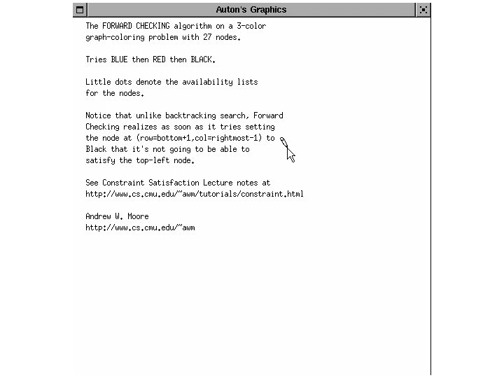
Forward Checking Algorithm V 3 V 4 V 2 V 6 V 5 V 1 R G • Initially, for each variable, record the set of all possible legal values for it • When you assign a value to a variable in the search, update the set of legal values for all unassigned variables. Backtrack immediately if you empty a variable’s set of possible values.

Forward Checking Algorithm – Keep track of remaining legal values for all variables – Deadend when any variable has no legal values

Example: Map-Coloring • Variables: WA, NT, Q, NSW, V, SA, T • Domains: Di = {red, green, blue} • Constraints: adjacent regions must have different colors e. g. , WA ≠ NT, or (WA, NT) in {(red, green), (red, blue), (green, red), (green, blue), (blue, red), (blue, green)}

Constraint Graph • Binary CSP: each constraint relates two variables • Constraint graph: nodes are variables, arcs are constraints

Forward Checking – Keep track of remaining legal values for all unassigned variables – Deadend when any variable has no legal values Note: WA is not the most constraining var

Forward Checking – Keep track of remaining legal values for all unassigned variables – Deadend when any variable has no legal values Note: Q is not most constrained variable

Forward Checking – Keep track of remaining legal values for all unassigned variables – Deadend when any variable has no legal values Note: V is not most constrained variable

Constraint Propagation • Forward checking propagates information from assigned to unassigned variables, but doesn't provide early detection for all failures: • NT and SA cannot both be blue! • Constraint propagation repeatedly (recursively) enforces constraints for all variables

Constraint Propagation V 3 V 5 V 2 V 6 V 4 V 1 R G Main idea: When you delete a value from a variable’s domain, check all variables connected to it. If any of them change, delete all inconsistent values connected to them, etc. Note: In the above example, nothing changes

Arc Consistency • Simplest form of propagation makes each arc (i. e. , each binary constraint) consistent • X Y is consistent if for every value x at var X there is some allowed y, i. e. , there is at least 1 value of Y that is consistent with x at X X = SA Y = NSW

Arc Consistency • Simplest form of propagation makes each arc consistent • X Y is consistent if for every value x at X there is some allowed y; if not, delete x X = NSW Y = SA

Arc Consistency • Simplest form of propagation makes each arc consistent • X Y is consistent if for every value x at X there is some allowed y; if not, delete x X=V Y = NSW • If X loses a value, all neighbors of X must be rechecked

Arc Consistency • Simplest form of propagation makes each arc consistent • X Y is consistent if for every value x at X there is some allowed y; if not, delete x X = SA Y = NT • If X loses a value, all neighbors of X must be rechecked • Arc consistency detects failure earlier than forward checking • Use as a preprocessor and after each assignment during search

Row 6, col 4 node must not be red because node to upperright (row 5, col 5) must not be black

Arc Consistency Algorithm “AC-3” function AC-3(csp) // returns false if inconsistency is found and true otherwise // input: csp, a binary CSP with components (X, D, C) // local variables: queue, a queue of arcs; initially all arcs in csp while queue not empty do { // check if Xi Xj consistent (Xi , Xj ) = Remove-First(queue); if Revise(csp, Xi , Xj ) then { // make arc consistent if size of Di = 0 then return false foreach Xk in Xi. Neighbors – { Xj } do // propagate changes to neighbors add (Xk , Xi ) to queue } } return true

Arc Consistency Algorithm “AC-3” function Revise(csp, Xi , Xj ) // returns true if we revise the domain of Xi revised = false; // check if Xi Xj consistent foreach x in Di do { if no value y in Dj allows (x, y) to satisfy the constraints between Xi and Xj then { delete x from Di ; revised = true; } } return revised

Constraint Propagation V 3 V 5 V 2 V 6 V 4 V 1 R G • In this example, constraint propagation solves the problem without search … But not always that lucky! • Constraint propagation can be done as a preprocessing step • And it can be performed during search – Note: when you backtrack, you must undo some of your additional constraints

Combining Search with CSP • Idea: Interleave search and CSP inference • Perform DFS – At each node assign a selected value to a selected variable – Run CSP to reduce variables’ domains and check if any inconsistencies arise as a result of this assignment

Combining Backtracking Search with CSP: MAC Algorithm function BACKTRACKING-SEARCH(csp) returns a solution or failure return BACKTRACK({ }, csp) function BACKTRACK(assignment, csp) returns a solution or failure if assignment is complete then return assignment; var = SELECT-UNASSIGNED-VARIABLE(csp); foreach value in ORDER-DOMAIN-VALUES(var, assignment, csp) do { if value is consistent with assignment then { add {var = value} to assignment; inferences = AC-3(csp, var, value); if inferences != failure then { add inferences to assignment; result = BACKTRACK(assignment, csp); if result != failure then return result; } } remove {var = value} and inferences from assignment; } return failure

Summary • CSPs are a special kind of problem: – states defined by values of a fixed set of variables – goal test defined by constraints on variable values • Backtracking = depth-first search with one variable assigned per node plus consistency checking • Variable ordering and value selection heuristics help significantly • Forward checking prevents assignments that guarantee later failure • Constraint propagation (e. g. , arc consistency) does additional work to constrain values and detect inconsistencies earlier