Constraint Satisfaction Problems Berlin Chen 2004 References 1

Constraint Satisfaction Problems Berlin Chen 2004 References: 1. S. Russell and P. Norvig. Artificial Intelligence: A Modern Approach. Chapter 5 2. S. Russell’s teaching materials

Introduction • Standard Search Problems – State is a “black box” with no discernible internal structure – Accessed by the goal test function, heuristic function, successor function, etc. • Constraint Satisfaction Problems (CSPs) – State and goal test conform to a standard, structured, and very Derive heuristics simple representation without domain-specific knowledge • State is defined by variables Xi with values vi from domain Di • Goal test is a set of constraints C 1, C 2, . . , Cm, which specifies allowable combinations of values for subsets of variables – Some CSPs require a solution that maximizes an objective function 2

Introduction (cont. ) • Consistency and completeness of a CSP – Consistent (or called legal) • Any assignment that does not violate any constraints – Complete • Every variable is assigned with a value • A solution to a CSP is a complete assignment satisfying all the constraints 3

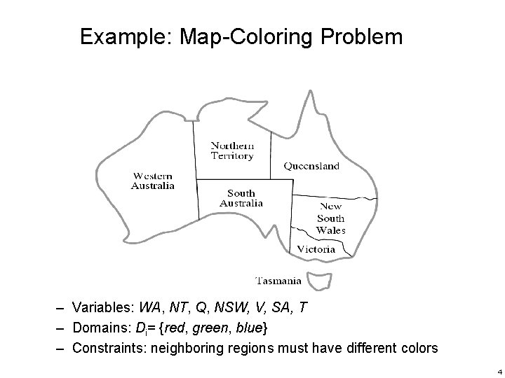
Example: Map-Coloring Problem – Variables: WA, NT, Q, NSW, V, SA, T – Domains: Di= {red, green, blue} – Constraints: neighboring regions must have different colors 4

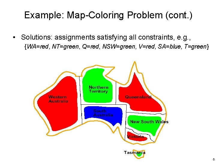
Example: Map-Coloring Problem (cont. ) • Solutions: assignments satisfying all constraints, e. g. , {WA=red, NT=green, Q=red, NSW=green, V=red, SA=blue, T=green} 5

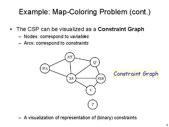
Example: Map-Coloring Problem (cont. ) • The CSP can be visualized as a Constraint Graph – Nodes: correspond to variables – Arcs: correspond to constraints Constraint Graph – A visualization of representation of (binary) constraints 6

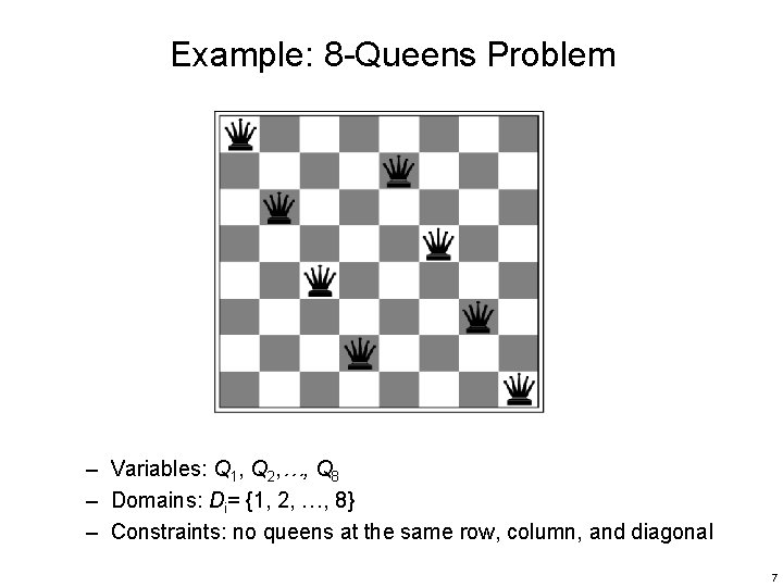
Example: 8 -Queens Problem – Variables: Q 1, Q 2, …, Q 8 – Domains: Di= {1, 2, …, 8} – Constraints: no queens at the same row, column, and diagonal 7

Benefits of CSPs • Conform the problem representation to a standard pattern – A set of variables with assigned values • Generic heuristics can be developed with no domainspecific expertise • The structure of constraint graph can be used to simplify the solution process – Exponential reduction 8

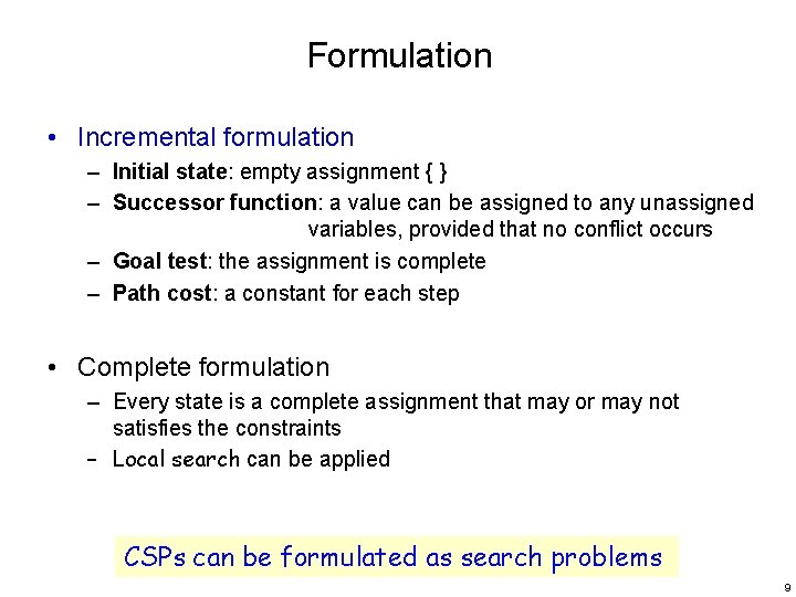
Formulation • Incremental formulation – Initial state: empty assignment { } – Successor function: a value can be assigned to any unassigned variables, provided that no conflict occurs – Goal test: the assignment is complete – Path cost: a constant for each step • Complete formulation – Every state is a complete assignment that may or may not satisfies the constraints – Local search can be applied CSPs can be formulated as search problems 9

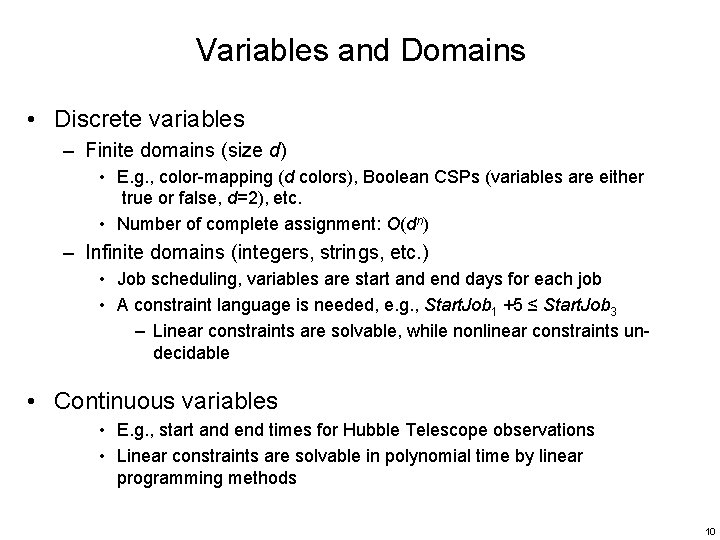
Variables and Domains • Discrete variables – Finite domains (size d) • E. g. , color-mapping (d colors), Boolean CSPs (variables are either true or false, d=2), etc. • Number of complete assignment: O(dn) – Infinite domains (integers, strings, etc. ) • Job scheduling, variables are start and end days for each job • A constraint language is needed, e. g. , Start. Job 1 +5 ≤ Start. Job 3 – Linear constraints are solvable, while nonlinear constraints undecidable • Continuous variables • E. g. , start and end times for Hubble Telescope observations • Linear constraints are solvable in polynomial time by linear programming methods 10

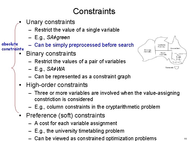
Constraints • Unary constraints absolute constraints – Restrict the value of a single variable – E. g. , SA≠green – Can be simply preprocessed before search • Binary constraints – Restrict the values of a pair of variables – E. g. , SA≠WA – Can be represented as a constraint graph • High-order constraints – Three or more variables are involved when the value-assigning constriction is considered – E. g. , column constraints in the cryptarithmetic problem • Preference (soft) constraints – A cost for each variable assignment – E. g. , the university timetabling problem – Can be viewed as constrained optimization problems 11

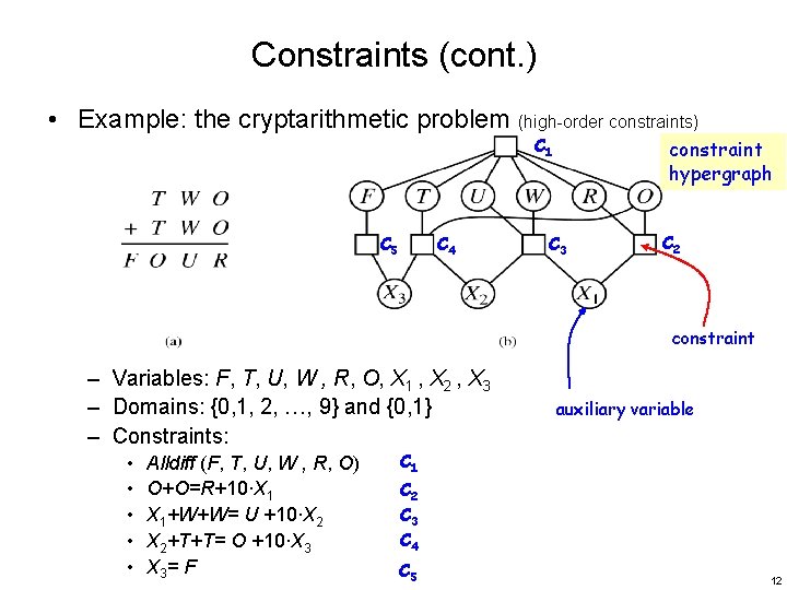
Constraints (cont. ) • Example: the cryptarithmetic problem (high-order constraints) C 1 C 5 C 4 constraint hypergraph C 3 C 2 constraint – Variables: F, T, U, W , R, O, X 1 , X 2 , X 3 – Domains: {0, 1, 2, …, 9} and {0, 1} – Constraints: • • • Alldiff (F, T, U, W , R, O) O+O=R+10∙X 1 X 1+W+W= U +10∙X 2 X 2+T+T= O +10∙X 3 X 3= F auxiliary variable C 1 C 2 C 3 C 4 C 5 12

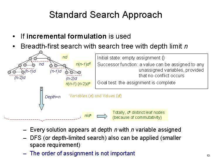
Standard Search Approach • If incremental formulation is used • Breadth-first search with search tree with depth limit n nd n(n-1)d 2 nd (n-1)d (n-2)d n(n-1) (n-2)d 3 Depth=n Initial state: empty assignment {} Successor function: a value can be assigned to any unassigned variables, provided that no conflict occurs Goal test: the assignment is complete Variables (n) and Values (d) n!dn Totally, dn distinct leaf nodes (because of commutativity) – Every solution appears at depth n with n variable assigned – DFS (or depth-limited search) also can be applied (smaller space requirement) – The order of assignment is not important 13

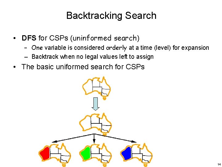
Backtracking Search • DFS for CSPs (uninformed search) – One variable is considered orderly at a time (level) for expansion – Backtrack when no legal values left to assign • The basic uniformed search for CSPs 14

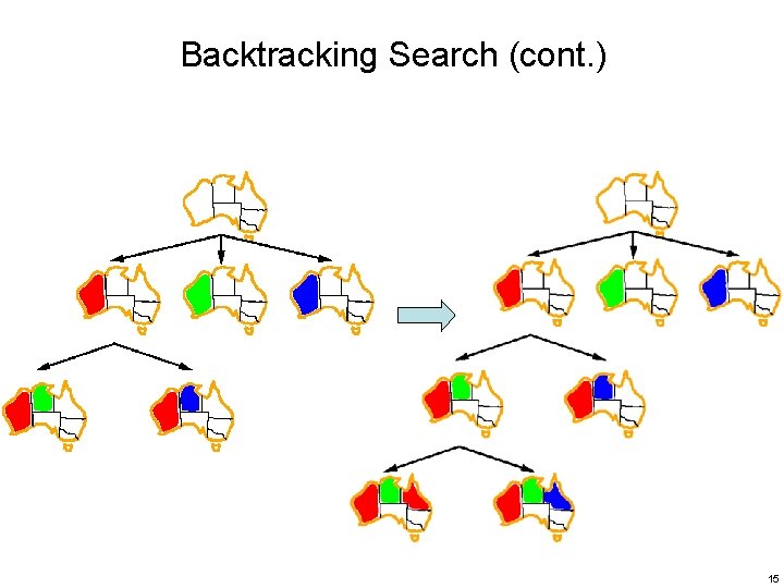
Backtracking Search (cont. ) 15

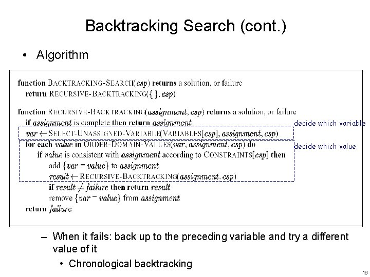
Backtracking Search (cont. ) • Algorithm decide which variable decide which value – When it fails: back up to the preceding variable and try a different value of it • Chronological backtracking 16

Improving Backtracking Efficiency • General-purpose methods help to speedup the search – What variable should be considered next? – In what order should variable’s values be tried? – Can we detect the inevitable failure early? – Can we take advantage of problem structure? 17

Improving Backtracking Efficiency (cont. ) • Variable Order – Minimum remaining value (MRV) • Also called ”most constrained variable”, “fail-first” – Degree heuristic • Act as a “tie-breaker” • Value Order – Least constraining value • If full search, value order does not matter • Propagate information through constraints – Forward checking – Constraint propagation 18

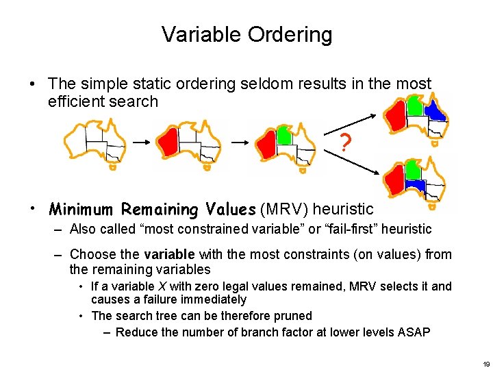
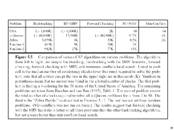
Variable Ordering • The simple static ordering seldom results in the most efficient search ? • Minimum Remaining Values (MRV) heuristic – Also called “most constrained variable” or “fail-first” heuristic – Choose the variable with the most constraints (on values) from the remaining variables • If a variable X with zero legal values remained, MRV selects it and causes a failure immediately • The search tree can be therefore pruned – Reduce the number of branch factor at lower levels ASAP 19

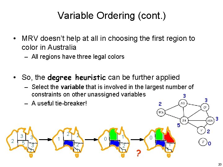
Variable Ordering (cont. ) • MRV doesn’t help at all in choosing the first region to color in Australia – All regions have three legal colors • So, the degree heuristic can be further applied – Select the variable that is involved in the largest number of constraints on other unassigned variables 3 – A useful tie-breaker! 2 5 2 3 5 3 3 2 1 2 2 2 1 0 1 2 1 0 ? 1 1 3 3 2 0 20

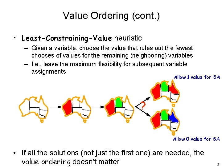
Value Ordering (cont. ) • Least-Constraining-Value heuristic – Given a variable, choose the value that rules out the fewest chooses of values for the remaining (neighboring) variables – I. e. , leave the maximum flexibility for subsequent variable assignments Allow 1 value for SA ? Allow 0 value for SA • If all the solutions (not just the first one) are needed, the value ordering doesn’t matter 21

22

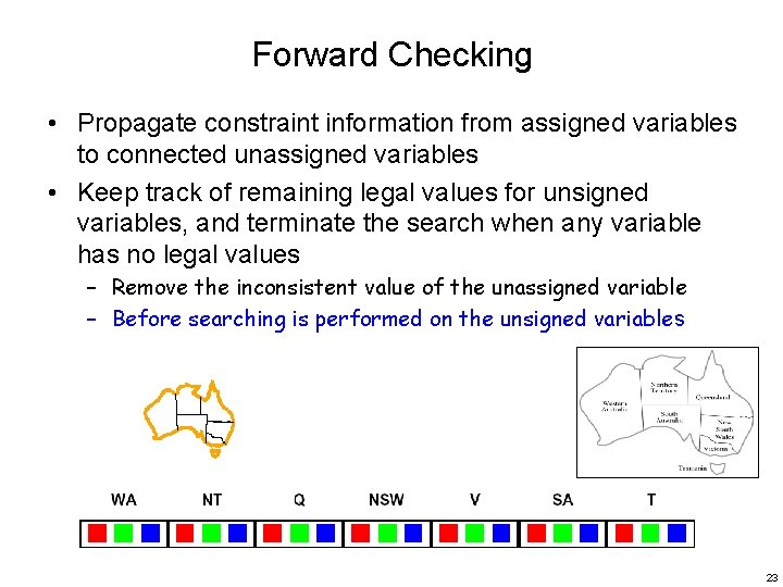
Forward Checking • Propagate constraint information from assigned variables to connected unassigned variables • Keep track of remaining legal values for unsigned variables, and terminate the search when any variable has no legal values – Remove the inconsistent value of the unassigned variable – Before searching is performed on the unsigned variables 23

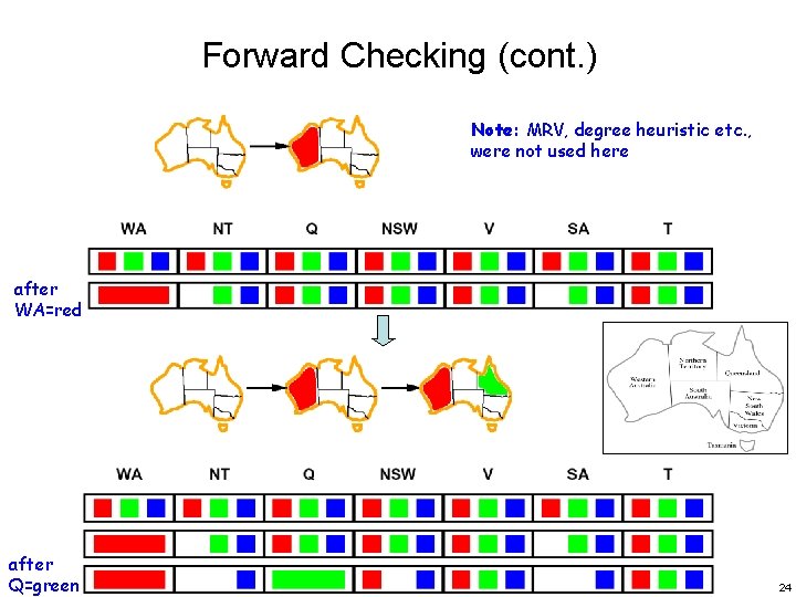
Forward Checking (cont. ) Note: MRV, degree heuristic etc. , were not used here after WA=red after Q=green 24

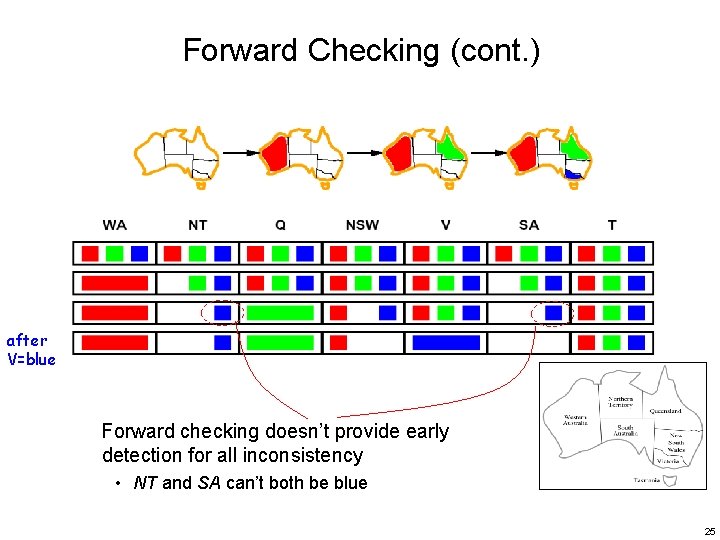
Forward Checking (cont. ) after V=blue Forward checking doesn’t provide early detection for all inconsistency • NT and SA can’t both be blue 25

Constraint Propagation • Repeated enforce constraints locally • Propagate the implications of a constraint on one variable onto other variables • Method – Arc consistency 26

Arc Consistency • X → Y is consistent iff for every value x of X there is some value y of Y that is consistent (allowable) – A method for implementing constraint propagation exists – Substantially stronger than forward checking 27

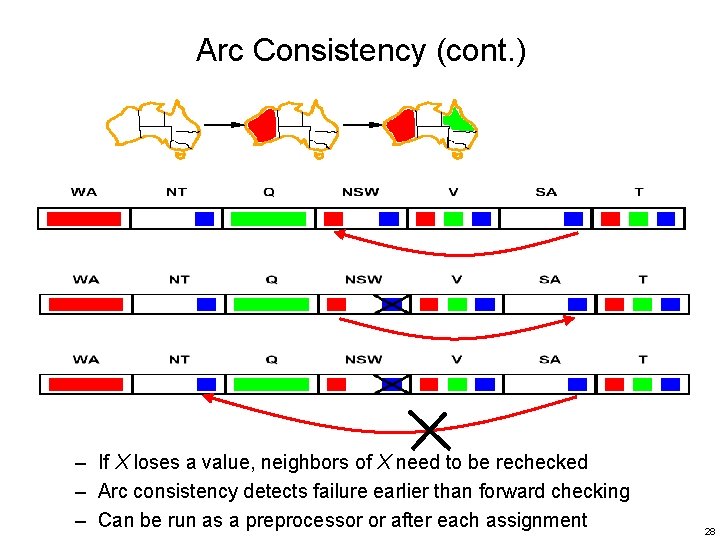
Arc Consistency (cont. ) – If X loses a value, neighbors of X need to be rechecked – Arc consistency detects failure earlier than forward checking – Can be run as a preprocessor or after each assignment 28

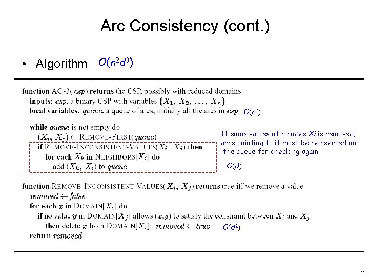
Arc Consistency (cont. ) • Algorithm O(n 2 d 3) O(n 2) If some values of a nodes Xi is removed, arcs pointing to it must be reinserted on the queue for checking again O(d) O(d 2) 29

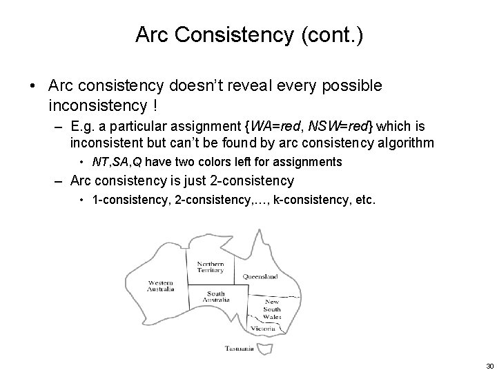
Arc Consistency (cont. ) • Arc consistency doesn’t reveal every possible inconsistency ! – E. g. a particular assignment {WA=red, NSW=red} which is inconsistent but can’t be found by arc consistency algorithm • NT, SA, Q have two colors left for assignments – Arc consistency is just 2 -consistency • 1 -consistency, 2 -consistency, …, k-consistency, etc. 30

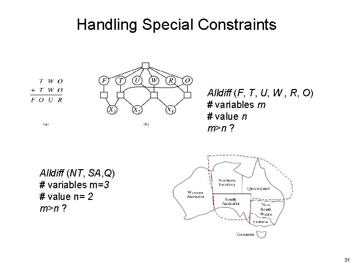
Handling Special Constraints Alldiff (F, T, U, W , R, O) # variables m # value n m>n ? Alldiff (NT, SA, Q) # variables m=3 # value n= 2 m>n ? 31

Local Search for CSPs • If complete formulation is used • Local search can easily be extended to CSPs with objection functions – Hill-climbing, simulated annealing etc. can be applied • Method – Allow states with unsatisfied constraints – Operators • reassign variable values – Variable selection • Randomly select any conflict variable – E. g. the “min-conflicts” heuristic • For a given variable, selecting the value that results the minimum number of conflicts with other variables • E. g. , hill-climbing with h(n)=total number of violated constraints 32

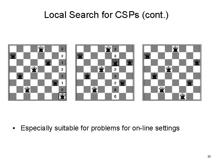
Local Search for CSPs (cont. ) • Especially suitable for problems for on-line settings 33

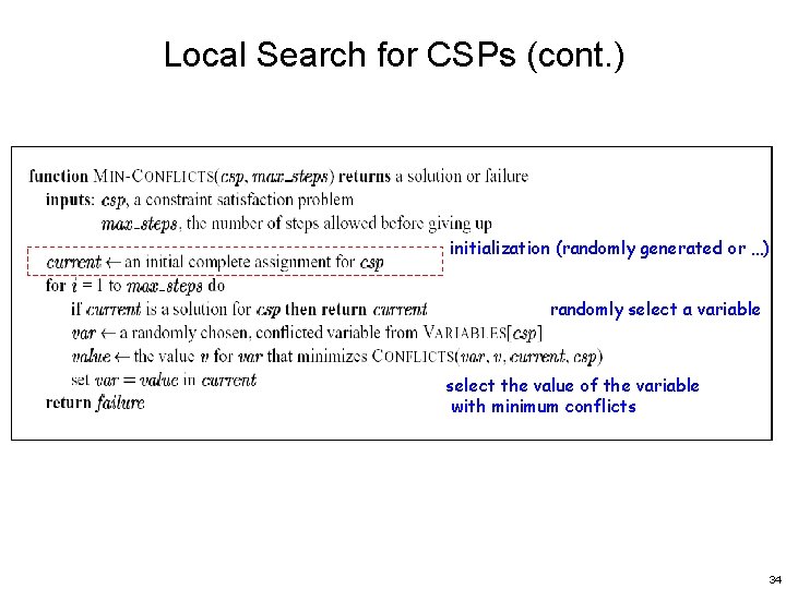
Local Search for CSPs (cont. ) initialization (randomly generated or …) randomly select a variable select the value of the variable with minimum conflicts 34

35

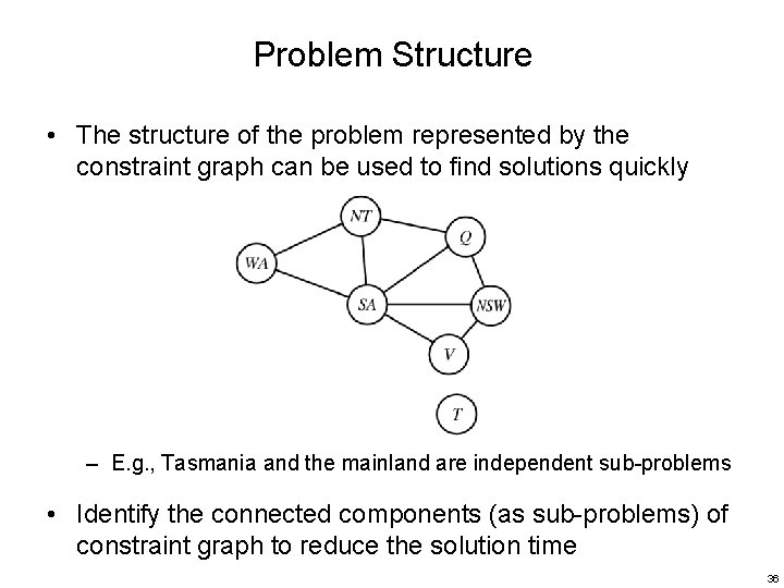
Problem Structure • The structure of the problem represented by the constraint graph can be used to find solutions quickly – E. g. , Tasmania and the mainland are independent sub-problems • Identify the connected components (as sub-problems) of constraint graph to reduce the solution time 36

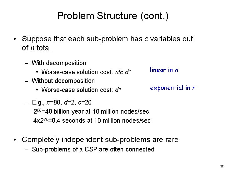
Problem Structure (cont. ) • Suppose that each sub-problem has c variables out of n total – With decomposition • Worse-case solution cost: n/c∙dc – Without decomposition • Worse-case solution cost: dn linear in n exponential in n – E. g. , n=80, d=2, c=20 280=40 billion year at 10 million nodes/sec 4 x 220=0. 4 seconds at 10 million nodes/sec • Completely independent sub-problems are rare – Sub-problems of a CSP are often connected 37

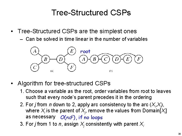
Tree-Structured CSPs • Tree-Structured CSPs are the simplest ones – Can be solved in time linear in the number of variables root • Algorithm for tree-structured CSPs 1. Choose a variable as the root, order variables from root to leaves such that every node’s parent precedes it in the ordering 2. For j from n down to 2, apply arc consistency to the arc (Xi, Xj), where Xi is the parent of Xj, remove the values from Domain[Xi] as necessary O(nd 2), if no loops 3. For j from 1 to n, assign Xj consistently with parent Xi 38

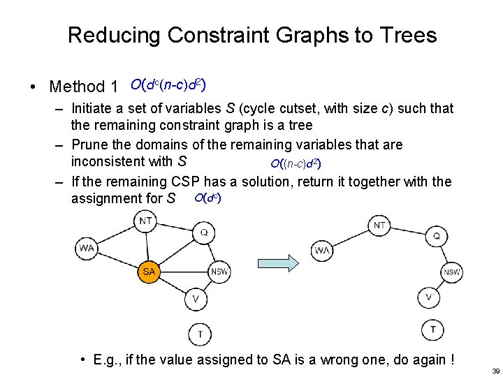
Reducing Constraint Graphs to Trees • Method 1 O(dc(n-c)d 2) – Initiate a set of variables S (cycle cutset, with size c) such that the remaining constraint graph is a tree – Prune the domains of the remaining variables that are inconsistent with S O((n-c)d 2) – If the remaining CSP has a solution, return it together with the assignment for S O(dc) • E. g. , if the value assigned to SA is a wrong one, do again ! 39

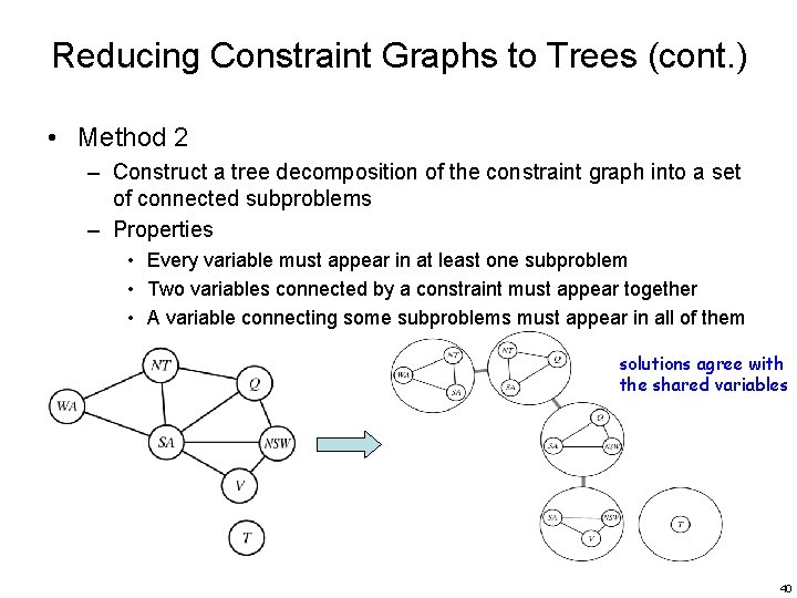
Reducing Constraint Graphs to Trees (cont. ) • Method 2 – Construct a tree decomposition of the constraint graph into a set of connected subproblems – Properties • Every variable must appear in at least one subproblem • Two variables connected by a constraint must appear together • A variable connecting some subproblems must appear in all of them solutions agree with the shared variables 40

41

42

43