Constraint propagation backtrackingbased search Roman Bartk Charles University

Constraint propagation backtracking-based search & Roman Barták Charles University, Prague (CZ) roman. bartak@mff. cuni. cz http: //ktiml. mff. cuni. cz/~bartak

„Constraint programming represents one of the closest approaches computer science has yet made to the Holy Grail of programming: the user states the problem, the computer solves it. “ Eugene C. Freuder, Constraints, April 1997 2

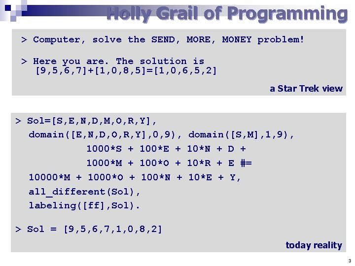
Holly Grail of Programming > Computer, solve the SEND, MORE, MONEY problem! > Here you are. The solution is [9, 5, 6, 7]+[1, 0, 8, 5]=[1, 0, 6, 5, 2] a Star Trek view > Sol=[S, E, N, D, M, O, R, Y], domain([E, N, D, O, R, Y], 0, 9), 1000*S + 100*E + 1000*M + 100*O + 10000*M + 1000*O + 100*N + all_different(Sol), labeling([ff], Sol). domain([S, M], 1, 9), 10*N + D + 10*R + E #= 10*E + Y, > Sol = [9, 5, 6, 7, 1, 0, 8, 2] today reality 3

Tutorial outline n Introduction ¨ n n history, applications, a constraint satisfaction problem Depth-first search ¨ backtracking, backjumping, backmarking ¨ incomplete and discrepancy search Consistency ¨ node, arc, and path consistencies ¨ k-consistency and global constraints Combining search and consistency ¨ look-back and look-ahead schemes ¨ variable and value ordering Conclusions ¨ constraint solvers, resources 4

Introduction

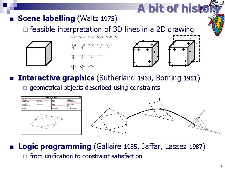
A bit of history n Scene labelling (Waltz 1975) ¨ feasible interpretation of 3 D lines in a 2 D drawing + - + + + n + + + - Interactive graphics (Sutherland 1963, Borning 1981) ¨ n + geometrical objects described using constraints Logic programming (Gallaire 1985, Jaffar, Lassez 1987) ¨ from unification to constraint satisfaction 6

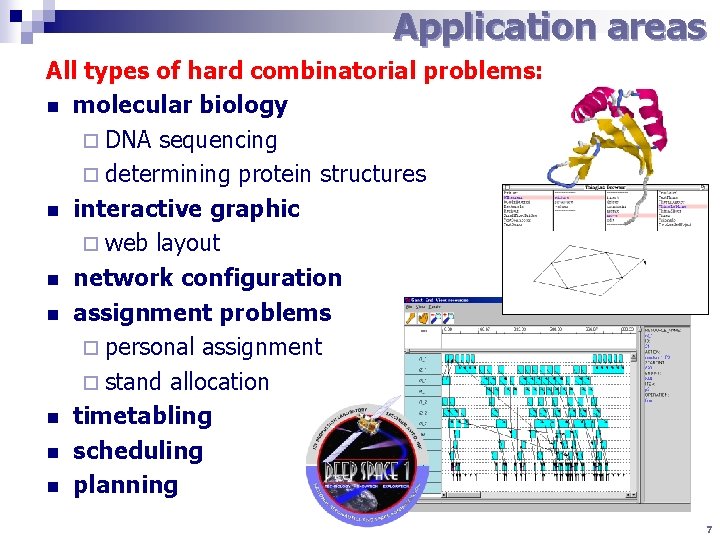
Application areas All types of hard combinatorial problems: n molecular biology ¨ DNA sequencing ¨ determining protein structures n interactive graphic ¨ web layout n network configuration n assignment problems ¨ personal assignment ¨ stand allocation n timetabling n scheduling n planning 7

Constraint technology based on declarative problem description via: ¨ variables with domains (sets of possible values) e. g. start of activity with time windows ¨ constraints restricting combinations of variables e. g. end. A < start. B constraint optimization via objective function e. g. minimize makespan Why to use constraint technology? ¨ understandable ¨ open and extendible ¨ proof of concept 8

CSP Constraint satisfaction problem consists of: ¨ a finite set of ¨ domains - a ¨ a finite set of variables finite set of values for each variable constraints n constraint is an arbitrary relation over the set of variables n can be defined extensionally (a set of compatible tuples) or intentionally (formula) A solution to a CSP is a complete consistent assignment of variables. ¨ complete = a value is assigned ¨ consistent = all the constraints to every variable are satisfied 9

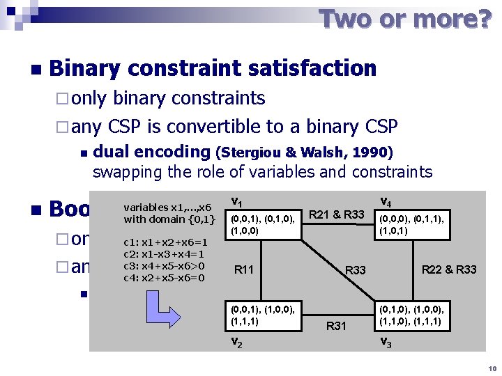
Two or more? n Binary constraint satisfaction ¨ only binary constraints ¨ any CSP is convertible to a binary CSP n n dual encoding (Stergiou & Walsh, 1990) swapping the role of variables and constraints v 1 v 4 (1, 0, 0) (1, 0, 1) Boolean constraint satisfaction (0, 0, 1), (0, 1, 0), R 21 & R 33 (0, 0, 0), (0, 1, 1), variables x 1, …, x 6 with domain {0, 1} ¨ only Boolean (two valued) domains c 1: x 1+x 2+x 6=1 c 2: x 1 -x 3+x 4=1 c 3: x 4+x 5 -x 6>0 ¨ any CSP is convertible R 11 to a Boolean R 33 CSP c 4: x 2+x 5 -x 6=0 n R 22 & R 33 SAT encoding (0, 0, 1), (1, 0, 0), (0, 1, 0), (1, 0, 0), Boolean variable indicates whether a given value is (1, 1, 1) (1, 1, 0), (1, 1, 1) R 31 assigned to the variable v v 2 3 10

Depth-first search

Basic idea n n We are looking for a complete consistent assignment! ¨ start with a consistent assignment (for example, empty one) ¨ extend the assignment towards a complete assignment Depth-first search is a technique of searching solution by extending a partial consistent assignment towards a complete consistent assignment. assign values gradually to variables ¨ after each assignment test consistency of the constraints over the assigned variables ¨ and backtrack upon failure ¨ n Backtracking is probably the most widely used complete systematic search algorithm. ¨ complete = guarantees finding a solution or proving its non-existence 12

Chronological backtracking A recursive definition procedure BT(X: variables, V: assignment, C: constraints) if X={} then return V x select a not-yet assigned variable from X for each value h from the domain of x do if consistent(V+{x/h}, C) then R BT(X-{x}, V+{x/h}, C) if R fail then return R end for return fail end BT call BT(X, {}, C) Consistency procedure checks satisfaction of constraints whose variables are already assigned. 13

Weaknesses of backtracking n thrashing ¨ throws away the reason of the conflict ¨ Example: A, B, C, D, E: : 1. . 10, A>E n BT tries all the assignments for B, C, D before finding that A 1 ¨ Solution: backjumping (jump to the source of the failure) n redundant work ¨ unnecessary constraint checks are repeated ¨ Example: A, B, C, D, E: : 1. . 10, B+8<D, C=5*E n when labelling C, E the values 1, . . , 9 are repeatedly checked for D ¨ Solution: backmarking, backchecking (remember (no-)good assignments) n late detection of the conflict ¨ constraint violation is discovered only when the values are known ¨ Example: A, B, C, D, E: : 1. . 10, A=3*E n the fact that A>2 is discovered when labelling E ¨ Solution: forward checking (forward check of constraints) 14

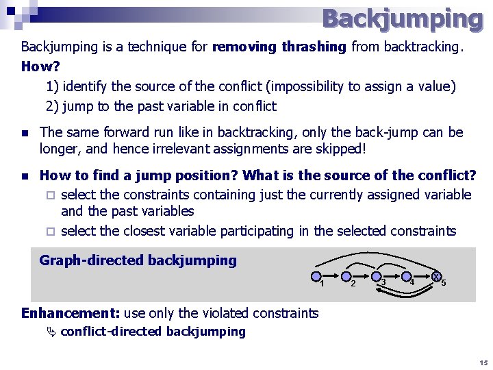
Backjumping is a technique for removing thrashing from backtracking. How? 1) identify the source of the conflict (impossibility to assign a value) 2) jump to the past variable in conflict n The same forward run like in backtracking, only the back-jump can be longer, and hence irrelevant assignments are skipped! n How to find a jump position? What is the source of the conflict? ¨ select the constraints containing just the currently assigned variable and the past variables ¨ select the closest variable participating in the selected constraints Graph-directed backjumping 1 2 3 4 x 5 Enhancement: use only the violated constraints conflict-directed backjumping 15

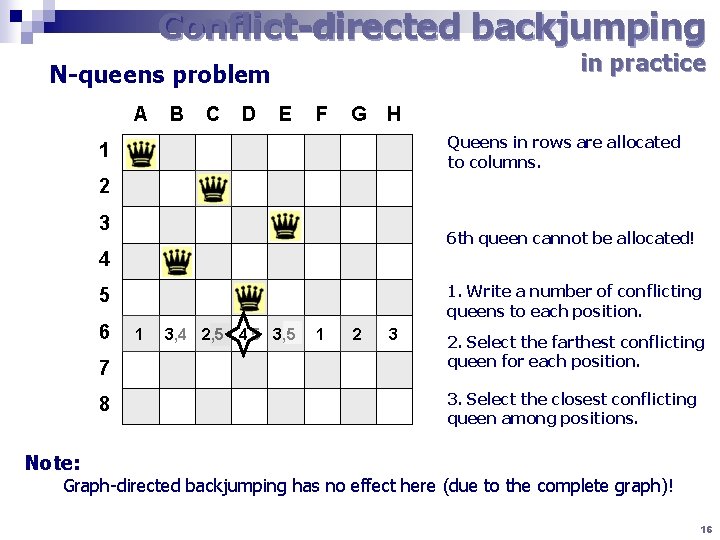
Conflict-directed backjumping in practice N-queens problem A B C D E F G H Queens in rows are allocated to columns. 1 2 3 6 th queen cannot be allocated! 4 1. Write a number of conflicting queens to each position. 5 6 7 8 1 3, 4 2, 5 4, 5 3, 5 1 2 3 2. Select the farthest conflicting queen for each position. 3. Select the closest conflicting queen among positions. Note: Graph-directed backjumping has no effect here (due to the complete graph)! 16

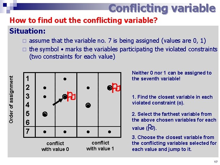
Conflicting variable How to find out the conflicting variable? Situation: assume that the variable no. 7 is being assigned (values are 0, 1) ¨ the symbol marks the variables participating the violated constraints (two constraints for each value) Order of assignment ¨ 1 2 3 4 5 6 7 Neither 0 nor 1 can be assigned to the seventh variable! 1. Find the closest variable in each violated constraint (o). 2. Select the farthest variable from the above chosen variables for each conflict with value 0 conflict with value 1 value ( ). 3. Choose the closest variable from the conflicting variables selected for each value and jump to it. 17

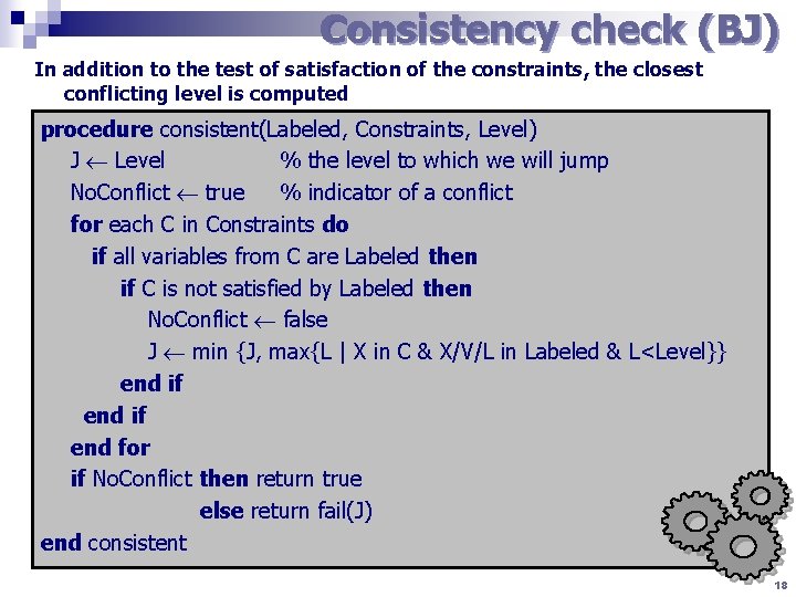
Consistency check (BJ) In addition to the test of satisfaction of the constraints, the closest conflicting level is computed procedure consistent(Labeled, Constraints, Level) J Level % the level to which we will jump No. Conflict true % indicator of a conflict for each C in Constraints do if all variables from C are Labeled then if C is not satisfied by Labeled then No. Conflict false J min {J, max{L | X in C & X/V/L in Labeled & L<Level}} end if end for if No. Conflict then return true else return fail(J) end consistent 18

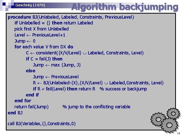
Gaschnig (1979) Algorithm backjumping procedure BJ(Unlabeled, Labeled, Constraints, Previous. Level) if Unlabelled = {} then return Labeled pick first X from Unlabelled Level Previous. Level+1 Jump 0 for each value V from DX do C consistent({X/V/Level} Labeled, Constraints, Level) if C = fail(J) then Jump max {Jump, J} else Jump Previous. Level R BJ(Unlabeled-{X}, {X/V/Level} Labeled, Constraints, Level) if R fail(Level) then return R % success or backjump end if end for return fail(Jump) % jump to the conflicting variable end BJ call BJ(Variables, {}, Constraints, 0) 19

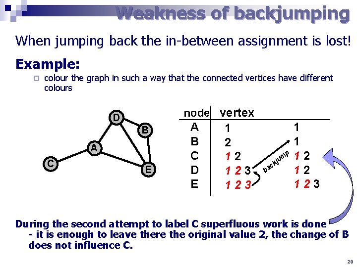
Weakness of backjumping When jumping back the in-between assignment is lost! Example: ¨ colour the graph in such a way that the connected vertices have different colours node vertex D B A C E A B C D E 1 2 12 123 1 1 2 p 12 m ju k c ba 12 123 During the second attempt to label C superfluous work is done - it is enough to leave there the original value 2, the change of B does not influence C. 20

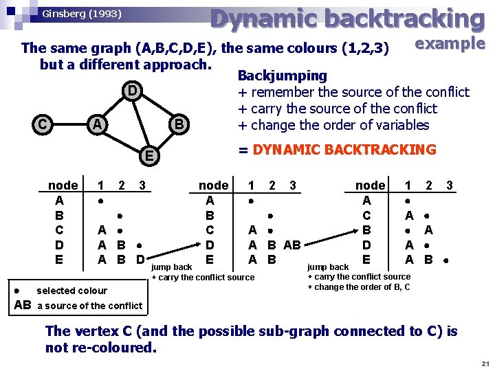
Dynamic backtracking Ginsberg (1993) example The same graph (A, B, C, D, E), the same colours (1, 2, 3) but a different approach. Backjumping D + remember the source of the conflict + carry the source of the conflict B C A + change the order of variables = DYNAMIC BACKTRACKING E node A B C D E AB 1 A A 2 3 B B D selected colour node A B C D E 1 A A jump back + carry the conflict source 2 3 B AB B node A C B D E 1 A A A jump back + carry the conflict source + change the order of B, C 2 3 A B a source of the conflict The vertex C (and the possible sub-graph connected to C) is not re-coloured. 21

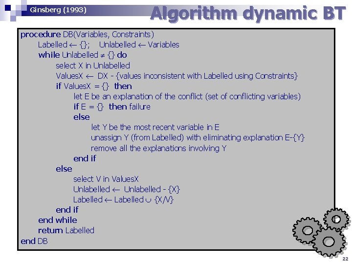
Ginsberg (1993) Algorithm dynamic BT procedure DB(Variables, Constraints) Labelled {}; Unlabelled Variables while Unlabelled {} do select X in Unlabelled Values. X DX - {values inconsistent with Labelled using Constraints} if Values. X = {} then let E be an explanation of the conflict (set of conflicting variables) if E = {} then failure else let Y be the most recent variable in E unassign Y (from Labelled) with eliminating explanation E-{Y} remove all the explanations involving Y end if else select V in Values. X Unlabelled - {X} Labelled {X/V} end if end while return Labelled end DB 22

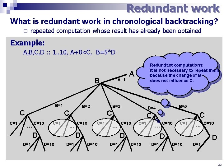
Redundant work What is redundant work in chronological backtracking? ¨ repeated computation whose result has already been obtained Example: A, B, C, D : : 1. . 10, A+8<C, B=5*D B B=1 C C=1 B=2 C=1 . . . D=1 C=10 C=1 D=10 D=1 C C. . . C=10 C=1 … C=10 D D=10 B=5 B=4 C D D A B=3 C. . . C=10 A=1 Redundant computations: it is not necessary to repeat them because the change of B does not influence C. D=1 C=1 . . . D D=10 D=1 C=10 D D=10 D=1 23

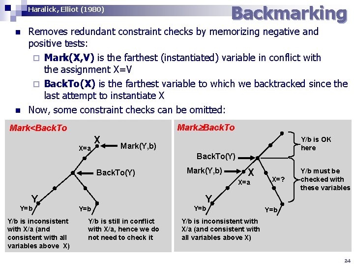
Backmarking Haralick, Elliot (1980) n n Removes redundant constraint checks by memorizing negative and positive tests: ¨ Mark(X, V) is the farthest (instantiated) variable in conflict with the assignment X=V ¨ Back. To(X) is the farthest variable to which we backtracked since the last attempt to instantiate X Now, some constraint checks can be omitted: Mark Back. To Mark<Back. To X=a X Y/b is OK here Mark(Y, b) Back. To(Y) Mark(Y, b) X X=a Y Y=b Y/b is inconsistent with X/a (and consistent with all variables above X) X=? Y/b must be checked with these variables Y Y=b Y/b is still in conflict with X/a, hence we do not need to check it Y=b Y/b is inconsistent with X/a (and consistent with all variables above X) 24

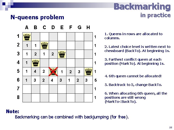
Backmarking in practice N-queens problem A B C D E F G H 1 1 2 1 1 3 1 2 4 1 5 1 6 7 8 1 1 1 2 1 1 4 3 2 2 1 4 3 2 1 2. Latest choice level is written next to chessboard (Back. To). At beginning 1 s. 3. Farthest conflict queen at each position (Mark. To). At beginning 1 s. 1 3 2 1. Queens in rows are allocated to columns. 4. 6 th queen cannot be allocated! 3 15 5. Backtrack to 5, change Back. To. 1 1 6. When allocating 6 th queen, all the positions are still wrong (Mark. To<Back. To). Note: Backmarking can be combined with backjumping (for free). 25

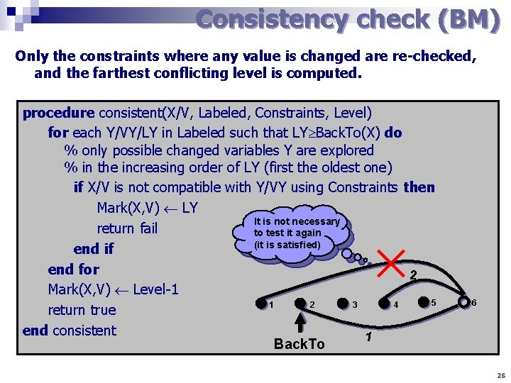
Consistency check (BM) Only the constraints where any value is changed are re-checked, and the farthest conflicting level is computed. procedure consistent(X/V, Labeled, Constraints, Level) for each Y/VY/LY in Labeled such that LY Back. To(X) do % only possible changed variables Y are explored % in the increasing order of LY (first the oldest one) if X/V is not compatible with Y/VY using Constraints then Mark(X, V) LY It is not necessary return fail to test it again (it is satisfied) end if end for 2 Mark(X, V) Level-1 5 1 2 3 4 return true end consistent 1 Back. To 6 26

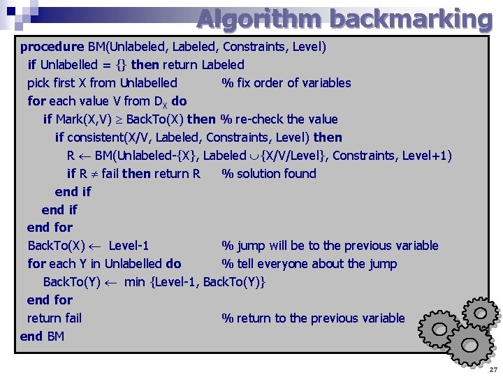
Algorithm backmarking procedure BM(Unlabeled, Labeled, Constraints, Level) if Unlabelled = {} then return Labeled pick first X from Unlabelled % fix order of variables for each value V from DX do if Mark(X, V) Back. To(X) then % re-check the value if consistent(X/V, Labeled, Constraints, Level) then R BM(Unlabeled-{X}, Labeled {X/V/Level}, Constraints, Level+1) if R fail then return R % solution found end if end for Back. To(X) Level-1 % jump will be to the previous variable for each Y in Unlabelled do % tell everyone about the jump Back. To(Y) min {Level-1, Back. To(Y)} end for return fail % return to the previous variable end BM 27

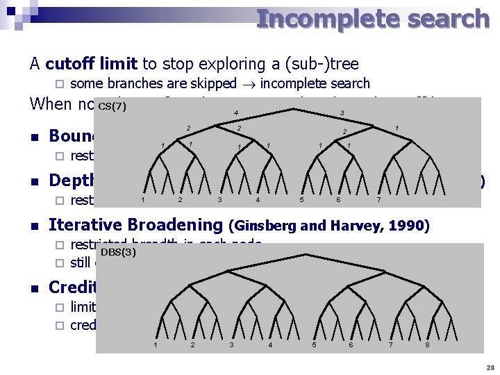
Incomplete search A cutoff limit to stop exploring a (sub-)tree ¨ some branches are skipped incomplete search IB(2) When no CS(7) solution found, restart with enlarged cutoff limit. 4 3 n 2 ¨ n 1 restricted number of backtracks Depth-bounded Backtrack Search (Cheadle et al. , 2003) 1 2 3 4 5 6 7 8 ¨ n 2 2 Bounded Backtrack Search (Harvey, 1995) 1 1 1 1 2 3 4 5 explored 6 restricted depth where alternatives are 7 Iterative Broadening (Ginsberg and Harvey, 1990) restricted breadth in each node BBS(8) DBS(3) ¨ still exponential! ¨ n Credit Search (Beldiceanu et al. , 1997) limited credit for exploring alternatives ¨ credit is split among the alternatives ¨ 1 12 3 4 5 26 7 8 93 4 5 6 7 8 28

Heuristics in search n Observation 1: n Heuristics - a guide of search The search space for real-life problems is so huge that it cannot be fully explored. they recommend a value for assignment ¨ quite often lead to a solution ¨ n What to do upon a failure of the heuristic? ¨ BT cares about the end of search (a bottom part of the search tree) so it rather repairs later assignments than the earliest ones thus BT assumes that the heuristic guides it well in the top part n Observation 2: n Observation 3: The heuristics are less reliable in the earlier parts of the search tree (as search proceeds, more information is available). The number of heuristic violations is usually small. 29

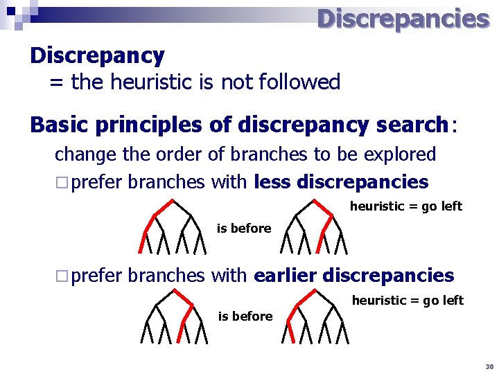
Discrepancies Discrepancy = the heuristic is not followed Basic principles of discrepancy search: change the order of branches to be explored ¨ prefer branches with less discrepancies heuristic = go left is before ¨ prefer branches with earlier discrepancies heuristic = go left is before 30

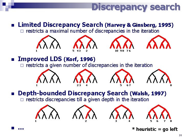
Discrepancy search n Limited Discrepancy Search (Harvey & Ginsberg, 1995) ¨ restricts a maximal number of discrepancies in the iteration 1 n 2 10 9 8 7 6 restricts a given number of discrepancies in the iteration 1 23 4 5 67 8 Depth-bounded Discrepancy Search (Walsh, 1997) ¨ restricts discrepancies till a given depth in the iteration 1 n 43 Improved LDS (Korf, 1996) ¨ n 5 … 2 3 4 5 6 7 8 * heuristic = go left 31

Consistency

Introduction to consistencies So far we used constraints in a passive way (as a test) … …in the best case we analysed the reason of the conflict. Cannot we use the constraints in a more active way? Example: A in 3. . 7, B in 1. . 5 A<B the variables’ domains the constraint many inconsistent values can be removed we get A in 3. . 4, B in 4. . 5 Note: it does not mean that all the remaining combinations of the values are consistent (for example A=4, B=4 is not consistent) How to remove the inconsistent values from the variables’ domains in the constraint network? 33

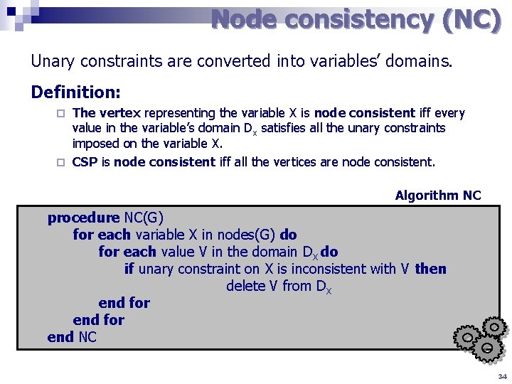
Node consistency (NC) Unary constraints are converted into variables’ domains. Definition: The vertex representing the variable X is node consistent iff every value in the variable’s domain Dx satisfies all the unary constraints imposed on the variable X. ¨ CSP is node consistent iff all the vertices are node consistent. ¨ Algorithm NC procedure NC(G) for each variable X in nodes(G) do for each value V in the domain DX do if unary constraint on X is inconsistent with V then delete V from DX end for end NC 34

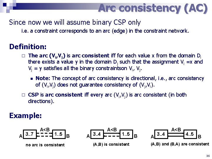
Arc consistency (AC) Since now we will assume binary CSP only i. e. a constraint corresponds to an arc (edge) in the constraint network. Definition: ¨ The arc (Vi, Vj) is arc consistent iff for each value x from the domain Di there exists a value y in the domain Dj such that the assignment Vi =x and Vj = y satisfies all the binary constraintson Vi, Vj. n ¨ Note: The concept of arc consistency is directional, i. e. , arc consistency of (Vi, Vj) does not guarantee consistency of (Vj, Vi). CSP is arc consistent iff every arc (Vi, Vj) is arc consistent (in both directions). Example: A 3. . 7 A<B 1. . 5 B no arc is consistent A 3. . 4 A<B 1. . 5 B (A, B) is consistent A 3. . 4 A<B 4. . 5 B (A, B) and (B, A) are consistent 35

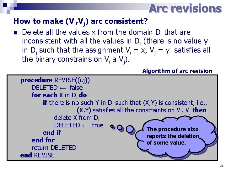
Arc revisions How to make (Vi, Vj) arc consistent? n Delete all the values x from the domain Di that are inconsistent with all the values in Dj (there is no value y in Dj such that the assignment Vi = x, Vj = y satisfies all the binary constrains on Vi a Vj). Algorithm of arc revision procedure REVISE((i, j)) DELETED false for each X in Di do if there is no such Y in Dj such that (X, Y) is consistent, i. e. , (X, Y) satisfies all the constraints on Vi, Vj then delete X from Di DELETED true The procedure also end if reports the deletion end for of some value. return DELETED end REVISE 36

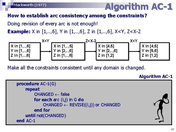
Algorithm AC-1 Mackworth (1977) How to establish arc consistency among the constraints? Doing revision of every arc is not enough! Example: X in [1, . . , 6], Y in [1, . . , 6], Z in [1, . . , 6], X<Y, Z<X-2 X<Y X in [1, . . , 6] Y in [1, . . , 6] Z<X-2 X in [1, . . , 5] Y in [2, . . , 6] Z in [1, . . , 6] X<Y X in [4, 5] Y in [2, . . , 6] Z in [1, 2] X in [4, 5] Y in [5, 6] Z in [1, 2] Make all the constraints consistent until any domain is changed. Algorithm AC-1 procedure AC-1(G) repeat CHANGED false for each arc (i, j) in G do CHANGED REVISE((i, j)) or CHANGED end for until not(CHANGED) end AC-1 37

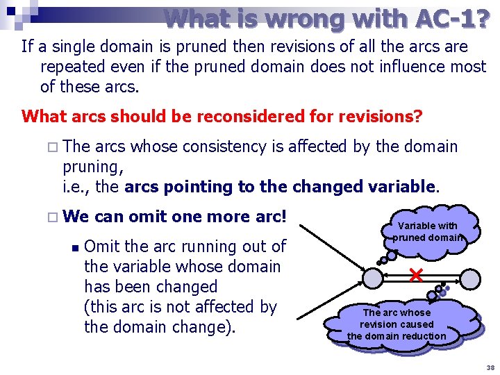
What is wrong with AC-1? If a single domain is pruned then revisions of all the arcs are repeated even if the pruned domain does not influence most of these arcs. What arcs should be reconsidered for revisions? ¨ The arcs whose consistency is affected by the domain pruning, i. e. , the arcs pointing to the changed variable. ¨ We n can omit one more arc! Omit the arc running out of the variable whose domain has been changed (this arc is not affected by the domain change). Variable with pruned domain The arc whose revision caused the domain reduction 38

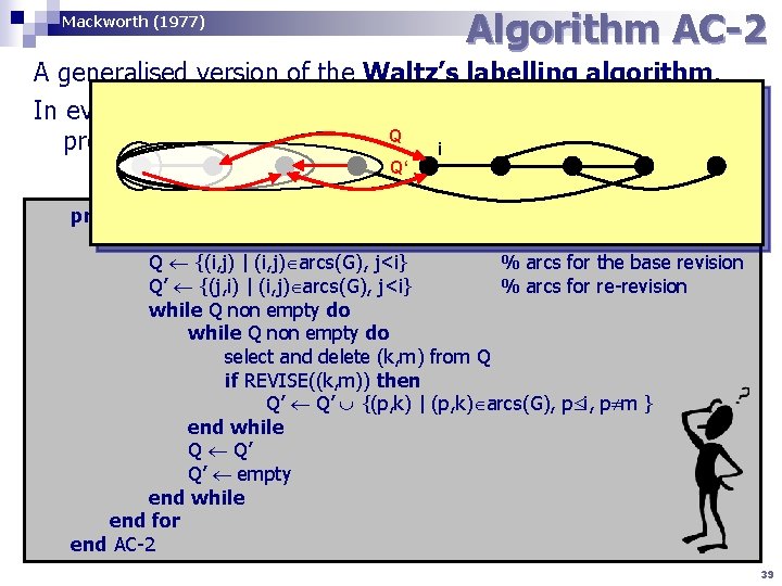
Algorithm AC-2 Mackworth (1977) A generalised version of the Waltz’s labelling algorithm. In every step, the arcs going back from a given vertex are Q visited nodes is AC) processed (i. e. a sub-graph of i Q‘ Algorithm AC-2 procedure AC-2(G) for i 1 to n do % n is a number of variables Q {(i, j) | (i, j) arcs(G), j<i} % arcs for the base revision Q’ {(j, i) | (i, j) arcs(G), j<i} % arcs for re-revision while Q non empty do select and delete (k, m) from Q if REVISE((k, m)) then Q’ {(p, k) | (p, k) arcs(G), p i, p m } end while Q Q’ Q’ empty end while end for end AC-2 39

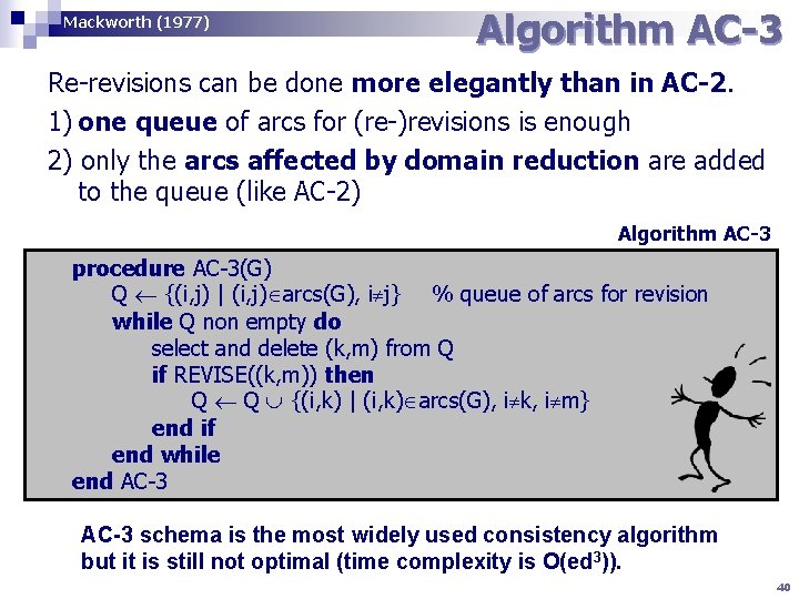
Mackworth (1977) Algorithm AC-3 Re-revisions can be done more elegantly than in AC-2. 1) one queue of arcs for (re-)revisions is enough 2) only the arcs affected by domain reduction are added to the queue (like AC-2) Algorithm AC-3 procedure AC-3(G) Q {(i, j) | (i, j) arcs(G), i j} % queue of arcs for revision while Q non empty do select and delete (k, m) from Q if REVISE((k, m)) then Q Q {(i, k) | (i, k) arcs(G), i k, i m} end if end while end AC-3 schema is the most widely used consistency algorithm but it is still not optimal (time complexity is O(ed 3)). 40

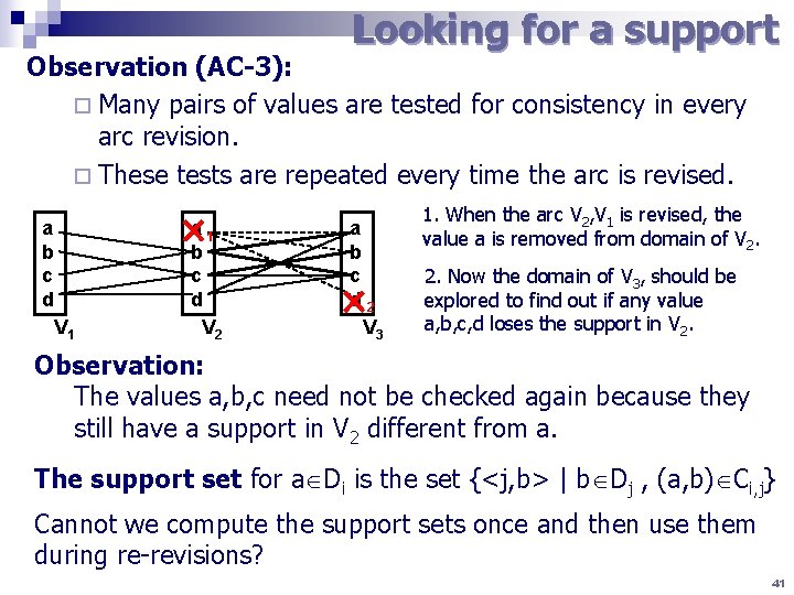
Looking for a support Observation (AC-3): ¨ Many pairs of values are tested for consistency in every arc revision. ¨ These tests are repeated every time the arc is revised. a b c d V 1 a 1 b c d V 2 a b c d 2 V 3 1. When the arc V 2, V 1 is revised, the value a is removed from domain of V 2. 2. Now the domain of V 3, should be explored to find out if any value a, b, c, d loses the support in V 2. Observation: The values a, b, c need not be checked again because they still have a support in V 2 different from a. The support set for a Di is the set {<j, b> | b Dj , (a, b) Ci, j} Cannot we compute the support sets once and then use them during re-revisions? 41

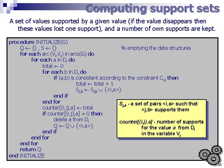
Computing support sets A set of values supported by a given value (if the value disappears then these values lost one support), and a number of own supports are kept. procedure INITIALIZE(G) Q {} , S {} % emptying the data structures for each arc (Vi, Vj) in arcs(G) do for each a in Di do total 0 for each b in Dj do if (a, b) is consistent according to the constraint Ci, j then total + 1 Sj, b {<i, a>} end if end for Sj, b - a set of pairs <i, a> such that counter[(i, j), a] total <j, b> supports them if counter[(i, j), a] = 0 then delete a from Di counter[(i, j), a] - number of supports Q Q {<i, a>} for the value a from Di end if in the variable Vj end for return Q end INITIALIZE 42

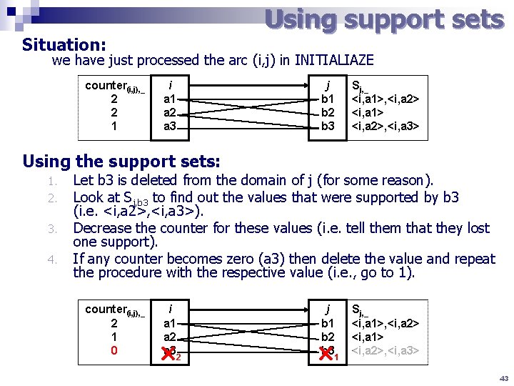
Using support sets Situation: we have just processed the arc (i, j) in INITIALIAZE counter(i, j), _ 2 2 1 i a 1 a 2 a 3 j b 1 b 2 b 3 Sj, _ <i, a 1>, <i, a 2> <i, a 1> <i, a 2>, <i, a 3> Using the support sets: 1. 2. 3. 4. Let b 3 is deleted from the domain of j (for some reason). Look at Sj, b 3 to find out the values that were supported by b 3 (i. e. <i, a 2>, <i, a 3>). Decrease the counter for these values (i. e. tell them that they lost one support). If any counter becomes zero (a 3) then delete the value and repeat the procedure with the respective value (i. e. , go to 1). counter(i, j), _ 2 2 1 1 0 i a 1 a 2 a 32 j b 1 b 2 b 31 Sj, _ <i, a 1>, <i, a 2> <i, a 1> <i, a 2>, <i, a 3> 43

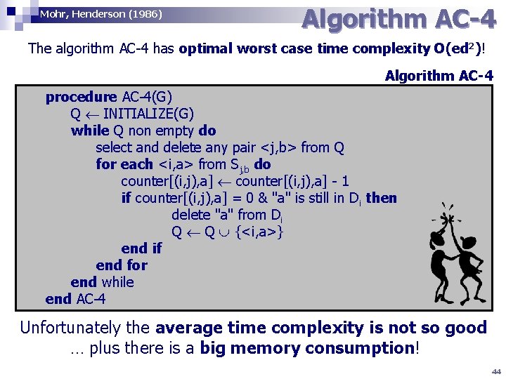
Mohr, Henderson (1986) Algorithm AC-4 The algorithm AC-4 has optimal worst case time complexity O(ed 2)! Algorithm AC-4 procedure AC-4(G) Q INITIALIZE(G) while Q non empty do select and delete any pair <j, b> from Q for each <i, a> from Sj, b do counter[(i, j), a] - 1 if counter[(i, j), a] = 0 & "a" is still in Di then delete "a" from Di Q Q {<i, a>} end if end for end while end AC-4 Unfortunately the average time complexity is not so good … plus there is a big memory consumption! 44

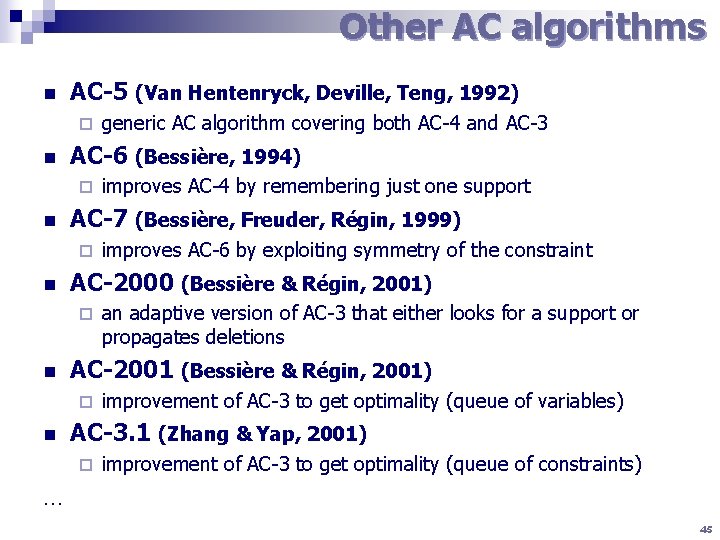
Other AC algorithms n AC-5 (Van Hentenryck, Deville, Teng, 1992) ¨ n AC-6 (Bessière, 1994) ¨ n an adaptive version of AC-3 that either looks for a support or propagates deletions AC-2001 (Bessière & Régin, 2001) ¨ n improves AC-6 by exploiting symmetry of the constraint AC-2000 (Bessière & Régin, 2001) ¨ n improves AC-4 by remembering just one support AC-7 (Bessière, Freuder, Régin, 1999) ¨ n generic AC algorithm covering both AC-4 and AC-3 improvement of AC-3 to get optimality (queue of variables) AC-3. 1 (Zhang & Yap, 2001) ¨ improvement of AC-3 to get optimality (queue of constraints) … 45

Directional arc consistency (DAC) Observation 1: AC has a directional character but a CSP is not directional. Observation 2: AC has to repeat arc revisions; the total number of revisions depends on the number of arcs but also on the size of domains (while cycle). Is it possible to weaken AC in such a way that every arc is revised just once? Definition: CSP is directional arc consistent using a given order of variables iff every arc (i, j) such that i<j is arc consistent. Again, every arc has to be revised, but revision in one direction is enough now. 46

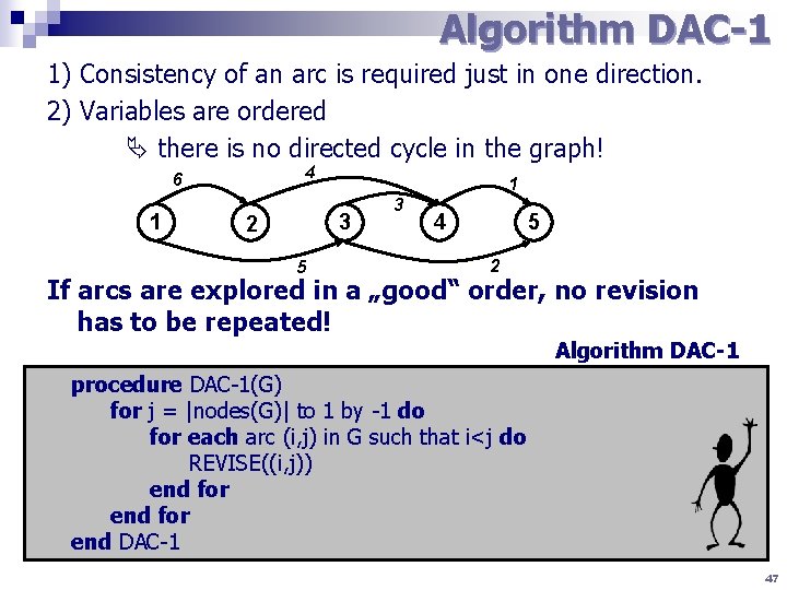
Algorithm DAC-1 1) Consistency of an arc is required just in one direction. 2) Variables are ordered there is no directed cycle in the graph! 4 6 1 1 3 2 5 3 4 5 2 If arcs are explored in a „good“ order, no revision has to be repeated! Algorithm DAC-1 procedure DAC-1(G) for j = |nodes(G)| to 1 by -1 do for each arc (i, j) in G such that i<j do REVISE((i, j)) end for end DAC-1 47

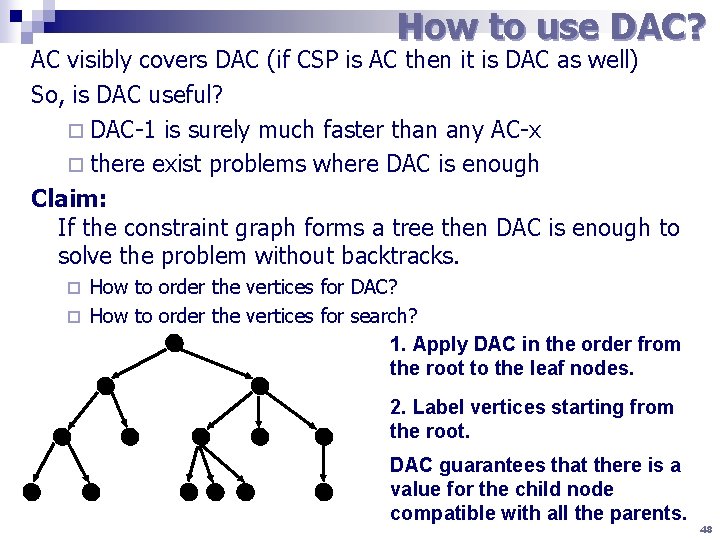
How to use DAC? AC visibly covers DAC (if CSP is AC then it is DAC as well) So, is DAC useful? ¨ DAC-1 is surely much faster than any AC-x ¨ there exist problems where DAC is enough Claim: If the constraint graph forms a tree then DAC is enough to solve the problem without backtracks. How to order the vertices for DAC? ¨ How to order the vertices for search? 1. Apply DAC in the order from the root to the leaf nodes. ¨ 2. Label vertices starting from the root. DAC guarantees that there is a value for the child node compatible with all the parents. 48

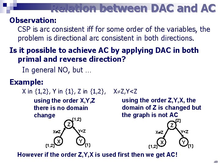
Relation between DAC and AC Observation: CSP is arc consistent iff for some order of the variables, the problem is directional arc consistent in both directions. Is it possible to achieve AC by applying DAC in both primal and reverse direction? In general NO, but … Example: X in {1, 2}, Y in {1}, Z in {1, 2}, using the order X, Y, Z there is no domain change {1, 2} X Z, Y<Z using the order Z, Y, X, the domain of Z is changed but the graph is not AC {2} Z X Z {1, 2} X Z Y<Z Y {1} X Z {1, 2} X Y<Z Y {1} However if the order Z, Y, X is used first then we get AC! 49

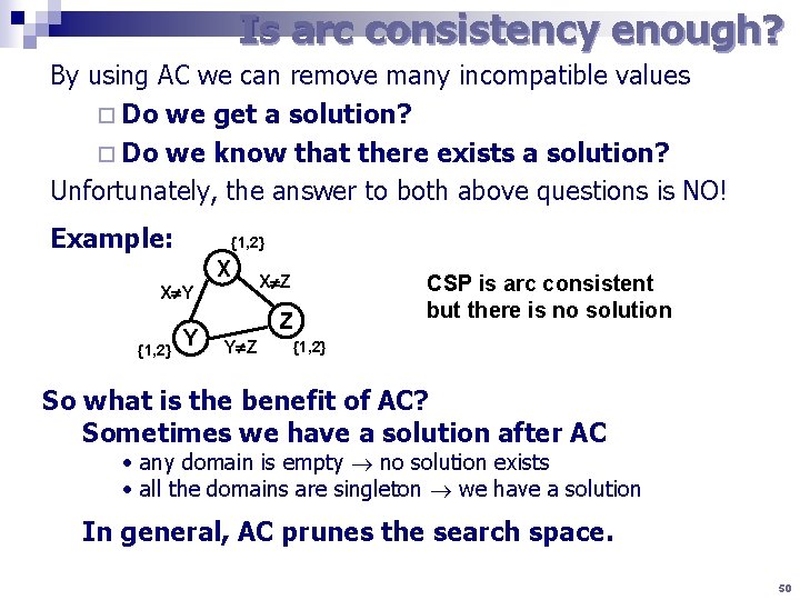
Is arc consistency enough? By using AC we can remove many incompatible values ¨ Do we get a solution? ¨ Do we know that there exists a solution? Unfortunately, the answer to both above questions is NO! Example: {1, 2} X X Y {1, 2} Y X Z Z Y Z CSP is arc consistent but there is no solution {1, 2} So what is the benefit of AC? Sometimes we have a solution after AC • any domain is empty no solution exists • all the domains are singleton we have a solution In general, AC prunes the search space. 50

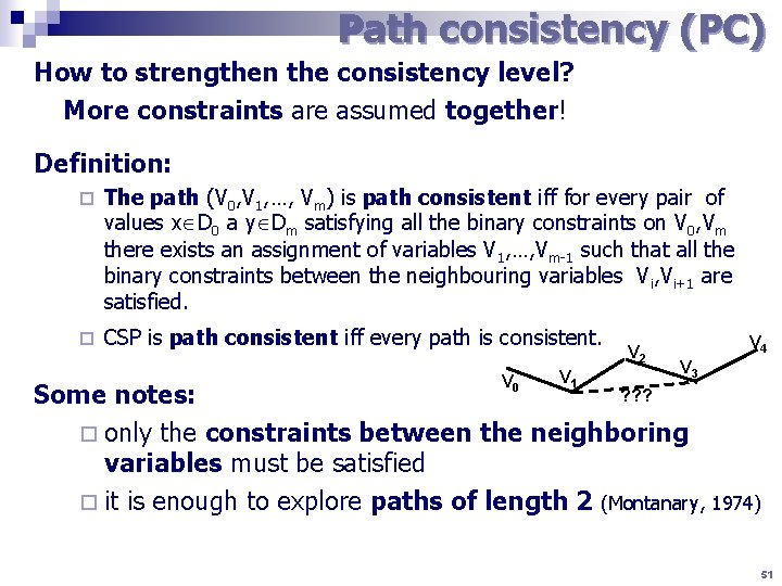
Path consistency (PC) How to strengthen the consistency level? More constraints are assumed together! Definition: ¨ The path (V 0, V 1, …, Vm) is path consistent iff for every pair of values x D 0 a y Dm satisfying all the binary constraints on V 0, Vm there exists an assignment of variables V 1, …, Vm-1 such that all the binary constraints between the neighbouring variables Vi, Vi+1 are satisfied. ¨ CSP is path consistent iff every path is consistent. V 0 V 1 V 2 V 4 V 3 ? ? ? Some notes: ¨ only the constraints between the neighboring variables must be satisfied ¨ it is enough to explore paths of length 2 (Montanary, 1974) 51

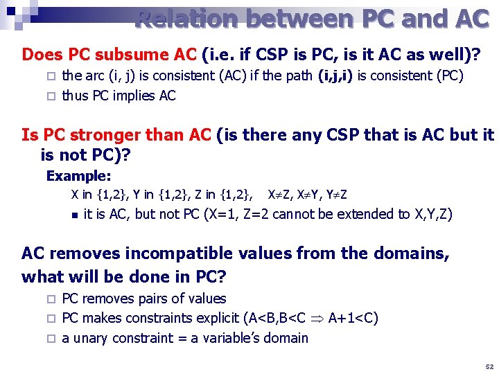
Relation between PC and AC Does PC subsume AC (i. e. if CSP is PC, is it AC as well)? the arc (i, j) is consistent (AC) if the path (i, j, i) is consistent (PC) ¨ thus PC implies AC ¨ Is PC stronger than AC (is there any CSP that is AC but it is not PC)? Example: X in {1, 2}, Y in {1, 2}, Z in {1, 2}, n X Z, X Y, Y Z it is AC, but not PC (X=1, Z=2 cannot be extended to X, Y, Z) AC removes incompatible values from the domains, what will be done in PC? PC removes pairs of values ¨ PC makes constraints explicit (A<B, B<C A+1<C) ¨ a unary constraint = a variable’s domain ¨ 52

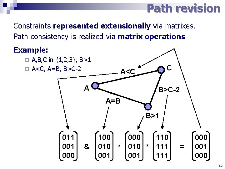
Path revision Constraints represented extensionally via matrixes. Path consistency is realized via matrix operations Example: A, B, C in {1, 2, 3}, B>1 ¨ A<C, A=B, B>C-2 ¨ C A<C A B>C-2 A=B B>1 011 000 & 100 000 110 010 * 111 001 111 = 000 001 000 53

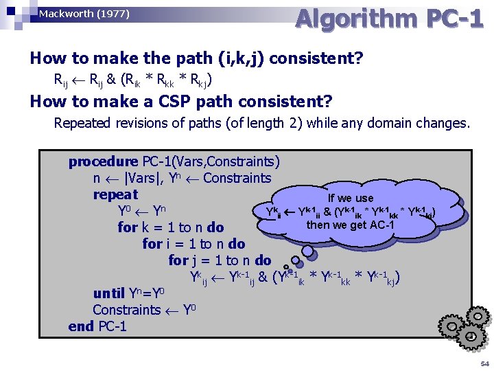
Mackworth (1977) Algorithm PC-1 How to make the path (i, k, j) consistent? Rij & (Rik * Rkj) How to make a CSP path consistent? Repeated revisions of paths (of length 2) while any domain changes. procedure PC-1(Vars, Constraints) n |Vars|, Yn Constraints repeat If we use 0 n Y Y Ykii Yk-1 ii & (Yk-1 ik * Yk-1 ki) then we get AC-1 for k = 1 to n do for i = 1 to n do for j = 1 to n do Ykij Yk-1 ij & (Yk-1 ik * Yk-1 kj) until Yn=Y 0 Constraints Y 0 end PC-1 54

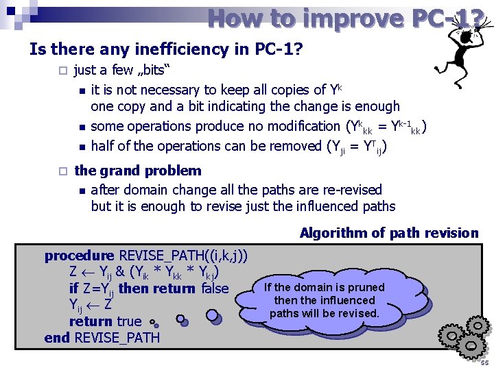
How to improve PC-1? Is there any inefficiency in PC-1? ¨ just a few „bits“ n it is not necessary to keep all copies of Y k one copy and a bit indicating the change is enough n some operations produce no modification (Y kkk = Yk-1 kk) n half of the operations can be removed (Y ji = YTij) ¨ the grand problem n after domain change all the paths are re-revised but it is enough to revise just the influenced paths Algorithm of path revision procedure REVISE_PATH((i, k, j)) Z Yij & (Yik * Ykj) if Z=Yij then return false Yij Z return true end REVISE_PATH If the domain is pruned then the influenced paths will be revised. 55

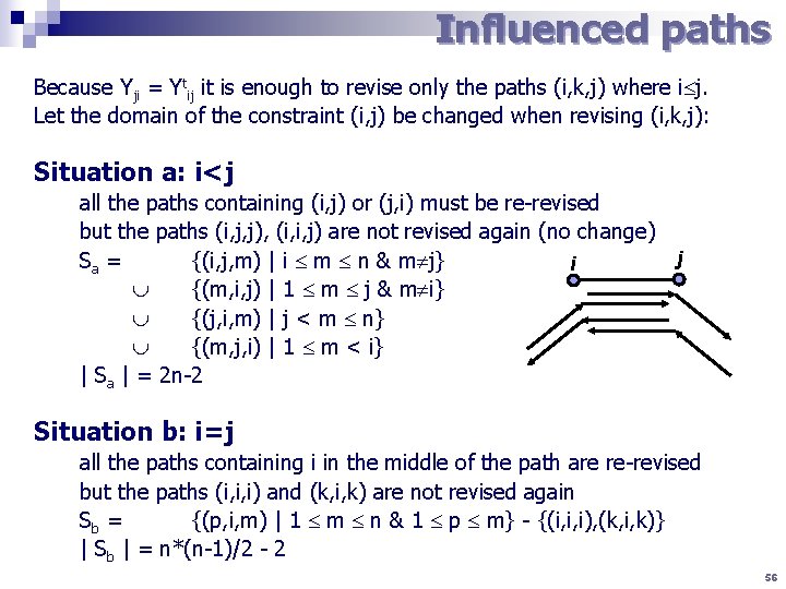
Influenced paths Because Yji = Ytij it is enough to revise only the paths (i, k, j) where i j. Let the domain of the constraint (i, j) be changed when revising (i, k, j): Situation a: i<j all the paths containing (i, j) or (j, i) must be re-revised but the paths (i, j, j), (i, i, j) are not revised again (no change) j Sa = {(i, j, m) | i m n & m j} i {(m, i, j) | 1 m j & m i} {(j, i, m) | j < m n} {(m, j, i) | 1 m < i} | Sa | = 2 n-2 Situation b: i=j all the paths containing i in the middle of the path are re-revised but the paths (i, i, i) and (k, i, k) are not revised again Sb = {(p, i, m) | 1 m n & 1 p m} - {(i, i, i), (k, i, k)} | Sb | = n*(n-1)/2 - 2 56

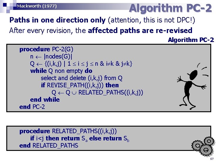
Mackworth (1977) Algorithm PC-2 Paths in one direction only (attention, this is not DPC!) After every revision, the affected paths are re-revised Algorithm PC-2 procedure PC-2(G) n |nodes(G)| Q {(i, k, j) | 1 i j n & i k & j k} while Q non empty do select and delete (i, k, j) from Q if REVISE_PATH((i, k, j)) then Q Q RELATED_PATHS((i, k, j)) end while end PC-2 procedure RELATED_PATHS((i, k, j)) if i<j then return Sa else return Sb end RELATED_PATHS 57

Other PC algorithms n PC-3 (Mohr, Henderson 1986) ¨ based on computing supports for a value (like AC-4) n If the pair (a, b) at the arc (i, j) is not supported by another variable, then a is removed from Di and b is removed from Dj. ¨ this algorithm is not sound! n PC-4 (Han, Lee 1988) ¨ correction of the PC-3 algorithm ¨ based on computing supports of pairs (b, c) at arc (i, j) n PC-5 (Singh 1995) ¨ uses the ideas behind AC-6 ¨ only one support is kept and a new support is looked for when the current support is lost 58

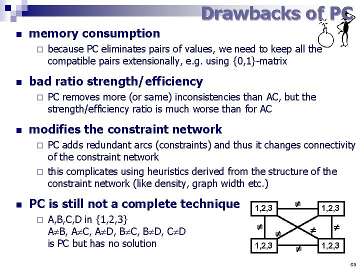
Drawbacks of PC n memory consumption ¨ n bad ratio strength/efficiency ¨ n because PC eliminates pairs of values, we need to keep all the compatible pairs extensionally, e. g. using {0, 1}-matrix PC removes more (or same) inconsistencies than AC, but the strength/efficiency ratio is much worse than for AC modifies the constraint network PC adds redundant arcs (constraints) and thus it changes connectivity of the constraint network ¨ this complicates using heuristics derived from the structure of the constraint network (like density, graph width etc. ) ¨ n PC is still not a complete technique ¨ A, B, C, D in {1, 2, 3} A B, A C, A D, B C, B D, C D is PC but has no solution 1, 2, 3 59

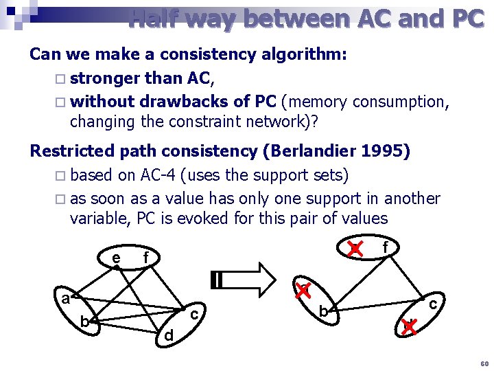
Half way between AC and PC Can we make a consistency algorithm: ¨ stronger than AC, ¨ without drawbacks of PC (memory consumption, changing the constraint network)? Restricted path consistency (Berlandier 1995) ¨ based on AC-4 (uses the support sets) ¨ as soon as a value has only one support in another variable, PC is evoked for this pair of values e e f a b c d a b f d c 60

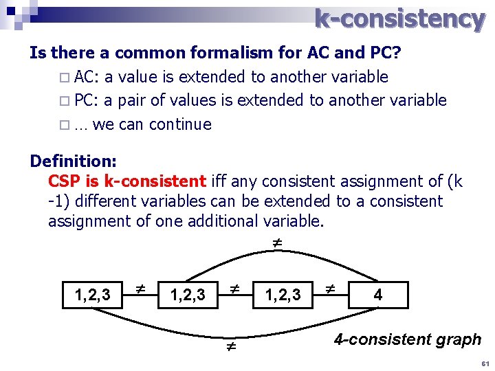
k-consistency Is there a common formalism for AC and PC? ¨ AC: a value is extended to another variable ¨ PC: a pair of values is extended to another variable ¨ … we can continue Definition: CSP is k-consistent iff any consistent assignment of (k -1) different variables can be extended to a consistent assignment of one additional variable. 1, 2, 3 4 4 -consistent graph 61

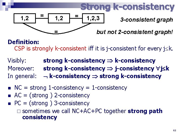
Strong k-consistency 1, 2 = = 1, 2, 3 3 -consistent graph but not 2 -consistent graph! Definition: CSP is strongly k-consistent iff it is j-consistent for every j k. Visibly: Moreover: In general: n n n strong k-consistency j-consistency j k k-consistency strong k-consistency NC = strong 1 -consistency = 1 -consistency AC = (strong ) 2 -consistency PC = (strong ) 3 -consistency ¨ sometimes we call NC+AC+PC together strong path consistency 62

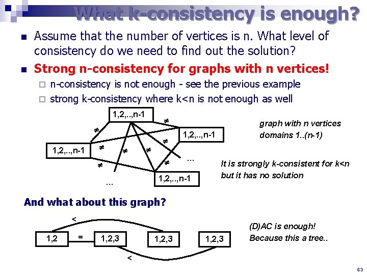
What k-consistency is enough? n n Assume that the number of vertices is n. What level of consistency do we need to find out the solution? Strong n-consistency for graphs with n vertices! n-consistency is not enough - see the previous example ¨ strong k-consistency where k<n is not enough as well ¨ 1, 2, . . , n-1 1, 2, . . , n-1 … graph with n vertices domains 1. . (n-1) It is strongly k-consistent for k<n but it has no solution And what about this graph? < 1, 2 = 1, 2, 3 (D)AC is enough! Because this a tree. . < 63

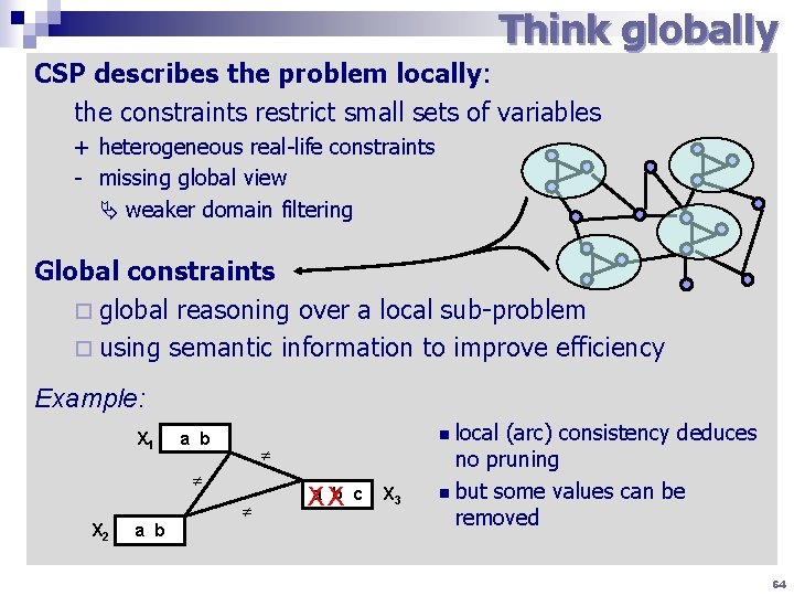
Think globally CSP describes the problem locally: the constraints restrict small sets of variables + heterogeneous real-life constraints - missing global view weaker domain filtering Global constraints ¨ global reasoning over a local sub-problem ¨ using semantic information to improve efficiency Example: X 1 a b X 2 a b local (arc) consistency deduces no pruning n but some values can be removed n b c Xa X X 3 64

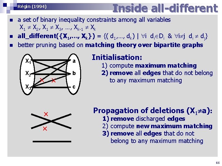
Inside all-different Régin (1994) n n n a set of binary inequality constraints among all variables X 1 X 2, X 1 X 3, …, Xk-1 Xk all_different({X 1, …, Xk}) = {( d 1, …, dk) | i di Di & i j di dj} better pruning based on matching theory over bipartite graphs X 11 X a X 22 X b X 33 X c Initialisation: 1) compute maximum matching 2) remove all edges that do not belong to any maximum matching Propagation of deletions (X 1 a): 1) remove discharged edges 2) compute new maximum matching 3) remove all edges that do not belong to any maximum matching 65

Search and Propagation

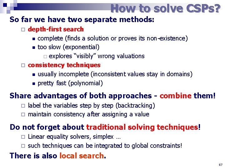
How to solve CSPs? So far we have two separate methods: depth-first search n complete (finds a solution or proves its non-existence) n too slow (exponential) ¨ explores “visibly” wrong valuations ¨ consistency techniques n usually incomplete (inconsistent values stay in domains) n pretty fast (polynomial) ¨ Share advantages of both approaches - combine them! label the variables step by step (backtracking) ¨ maintain consistency after assigning a value ¨ Do not forget about traditional solving techniques! Linear equality solvers, simplex … ¨ such techniques can be integrated to global constraints! ¨ There is also local search. 67

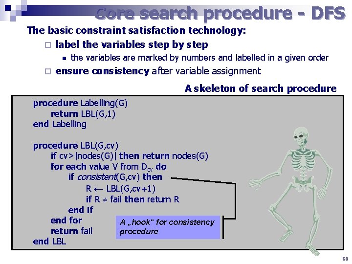
Core search procedure - DFS The basic constraint satisfaction technology: ¨ label the variables step by step n ¨ the variables are marked by numbers and labelled in a given order ensure consistency after variable assignment A skeleton of search procedure Labelling(G) return LBL(G, 1) end Labelling procedure LBL(G, cv) if cv>|nodes(G)| then return nodes(G) for each value V from Dcv do if consistent(G, cv) then R LBL(G, cv+1) if R fail then return R end if end for A „hook“ for consistency return fail procedure end LBL 68

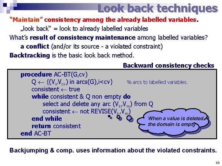
Look back techniques “Maintain” consistency among the already labelled variables. „look back“ = look to already labelled variables What’s result of consistency maintenance among labelled variables? a conflict (and/or its source - a violated constraint) Backtracking is the basic look back method. Backward consistency checks procedure AC-BT(G, cv) Q {(Vi, Vcv) in arcs(G), i<cv} % arcs to labelled variables. consistent true while consistent & Q non empty do select and delete any arc (Vk, Vm) from Q consistent not REVISE(Vk, Vm) When a value is deleted, end while the domain is empty return consistent end AC-BT Backjumping & comp. uses information about the violated constraints. 69

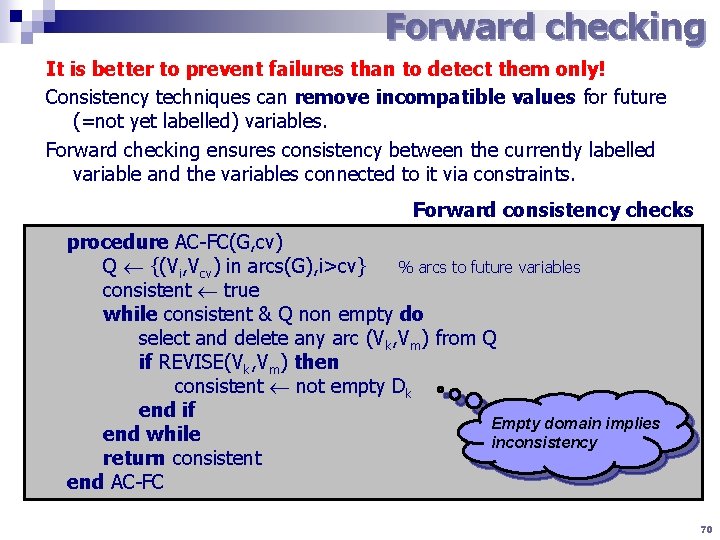
Forward checking It is better to prevent failures than to detect them only! Consistency techniques can remove incompatible values for future (=not yet labelled) variables. Forward checking ensures consistency between the currently labelled variable and the variables connected to it via constraints. Forward consistency checks procedure AC-FC(G, cv) Q {(Vi, Vcv) in arcs(G), i>cv} % arcs to future variables consistent true while consistent & Q non empty do select and delete any arc (Vk, Vm) from Q if REVISE(Vk, Vm) then consistent not empty Dk end if Empty domain implies end while inconsistency return consistent end AC-FC 70

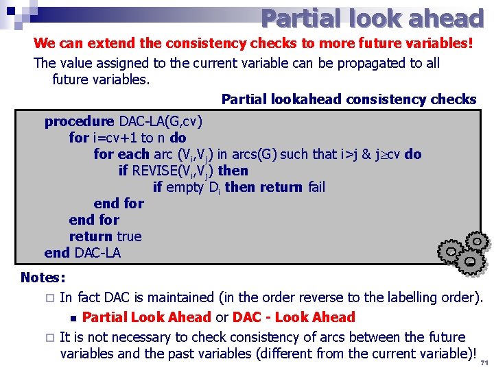
Partial look ahead We can extend the consistency checks to more future variables! The value assigned to the current variable can be propagated to all future variables. Partial lookahead consistency checks procedure DAC-LA(G, cv) for i=cv+1 to n do for each arc (Vi, Vj) in arcs(G) such that i>j & j cv do if REVISE(Vi, Vj) then if empty Di then return fail end for return true end DAC-LA Notes: ¨ In fact DAC is maintained (in the order reverse to the labelling order). n Partial Look Ahead or DAC - Look Ahead ¨ It is not necessary to check consistency of arcs between the future variables and the past variables (different from the current variable)! 71

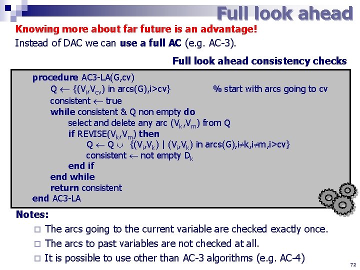
Full look ahead Knowing more about far future is an advantage! Instead of DAC we can use a full AC (e. g. AC-3). Full look ahead consistency checks procedure AC 3 -LA(G, cv) Q {(Vi, Vcv) in arcs(G), i>cv} % start with arcs going to cv consistent true while consistent & Q non empty do select and delete any arc (Vk, Vm) from Q if REVISE(Vk, Vm) then Q Q {(Vi, Vk) | (Vi, Vk) in arcs(G), i k, i m, i>cv} consistent not empty Dk end if end while return consistent end AC 3 -LA Notes: ¨ The arcs going to the current variable are checked exactly once. ¨ The arcs to past variables are not checked at all. ¨ It is possible to use other than AC-3 algorithms (e. g. AC-4) 72

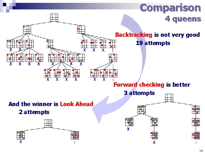
Comparison 4 queens Backtracking is not very good 19 attempts Forward checking is better 3 attempts And the winner is Look Ahead 2 attempts 73

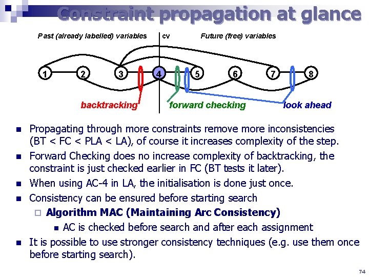
Constraint propagation at glance Past (already labelled) variables 1 2 3 backtracking n n n cv 4 Future (free) variables 5 6 forward checking 7 8 look ahead Propagating through more constraints remove more inconsistencies (BT < FC < PLA < LA), of course it increases complexity of the step. Forward Checking does no increase complexity of backtracking, the constraint is just checked earlier in FC (BT tests it later). When using AC-4 in LA, the initialisation is done just once. Consistency can be ensured before starting search ¨ Algorithm MAC (Maintaining Arc Consistency) n AC is checked before search and after each assignment It is possible to use stronger consistency techniques (e. g. use them once before starting search). 74

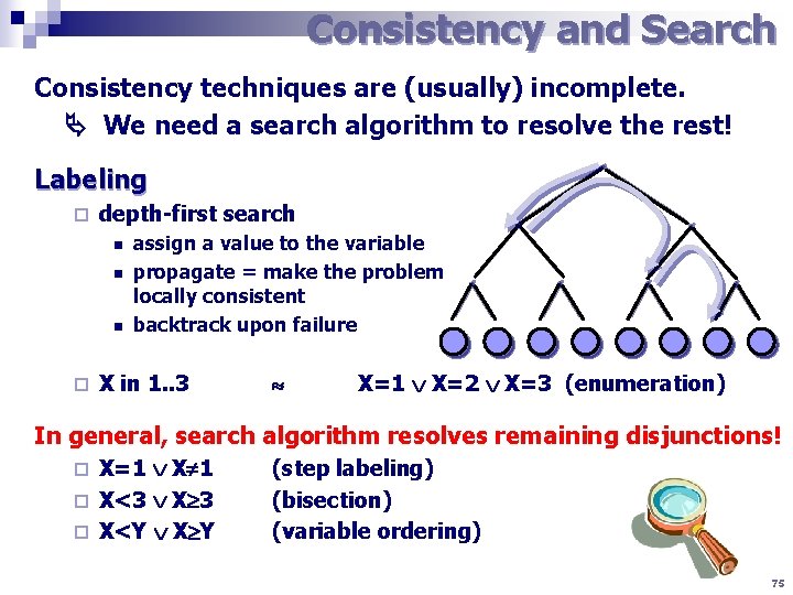
Consistency and Search Consistency techniques are (usually) incomplete. We need a search algorithm to resolve the rest! Labeling ¨ depth-first search n n n ¨ assign a value to the variable propagate = make the problem locally consistent backtrack upon failure X in 1. . 3 X=1 X=2 X=3 (enumeration) In general, search algorithm resolves remaining disjunctions! X=1 X 1 ¨ X<3 X 3 ¨ X<Y X Y ¨ (step labeling) (bisection) (variable ordering) 75

Variable ordering in labelling influence significantly efficiency of solvers (e. g. in a tree-structured CSP). What variable ordering should be chosen in general? FAIL-FIRST principle „select the variable whose instantiation will lead to a failure“ it is better to tackle failures earlier, they can be become even harder ¨ prefer the variables with smaller domain (dynamic order) n n a smaller number of choices ~ lower probability of success the dynamic order is appropriate only when new information appears during solving (e. g. , in look ahead algorithms) „solve the hard cases first, they may become even harder later“ ¨ prefer the most constrained variables n it is more complicated to label such variables (it is possible to assume complexity of satisfaction of the constraints) n this heuristic is used when there is an equal size of the domains ¨ prefer the variables with more constraints to past variables n a static heuristic that is useful for look-back techniques 76

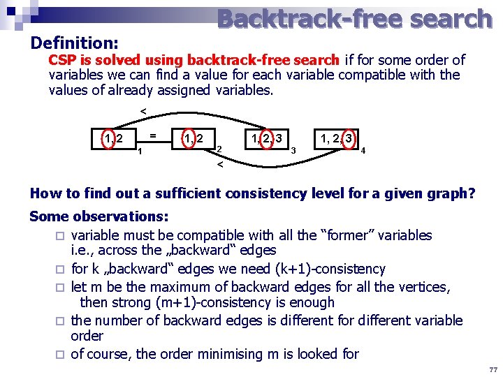
Backtrack-free search Definition: CSP is solved using backtrack-free search if for some order of variables we can find a value for each variable compatible with the values of already assigned variables. < = 1, 2 1 1, 2 2 1, 2, 3 3 4 < How to find out a sufficient consistency level for a given graph? Some observations: ¨ variable must be compatible with all the “former” variables i. e. , across the „backward“ edges ¨ for k „backward“ edges we need (k+1)-consistency ¨ let m be the maximum of backward edges for all the vertices, then strong (m+1)-consistency is enough ¨ the number of backward edges is different for different variable order ¨ of course, the order minimising m is looked for 77

Value ordering Order of values in labelling influence significantly efficiency (if we choose the right value each time, no backtrack is necessary). What value ordering for the variable should be chosen in general? SUCCEED FIRST principle „prefer the values belonging to the solution“ ¨ if no value is part of the solution then we have to check all values ¨ if there is a value from the solution then it is better to find it soon Note: SUCCEED FIRST does not go against FIRST-FAIL ! ¨ prefer the values with more suppors n this information can be found in AC-4 ¨ prefer the value leading to less domain reduction n this information can be computed usingleton consistency ¨ prefer the value simplifying the problem n solve approximation of the problem (e. g. a tree) Generic heuristics are usually too complex for computation. It is better to use problem-driven heuristics that propose the value! 78

Example

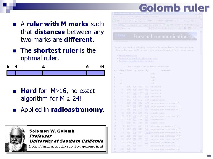
Golomb ruler 0 n A ruler with M marks such that distances between any two marks are different. n The shortest ruler is the optimal ruler. 1 4 9 11 n Hard for M 16, no exact algorithm for M 24! n Applied in radioastronomy. Solomon W. Golomb Professor University of Southern California http: //csi. usc. edu/faculty/golomb. html 80

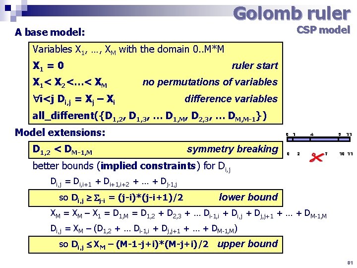
Golomb ruler CSP model A base model: Variables X 1, …, XM with the domain 0. . M*M X 1 = 0 X 1< X 2<…< XM ruler start no permutations of variables i<j Di, j = Xj – Xi difference variables all_different({D 1, 2, D 1, 3, … D 1, M, D 2, 3, … DM, M-1}) Model extensions: D 1, 2 < DM-1, M 0 1 symmetry breaking better bounds (implied constraints) for Di, j 0 4 2 9 7 11 10 11 Di, j = Di, i+1 + Di+1, i+2 + … + Dj-1, j so Di, j j-i = (j-i)*(j-i+1)/2 lower bound XM = XM – X 1 = D 1, M = D 1, 2 + D 2, 3 + … Di-1, i + Di, j + Dj, j+1 + … + DM-1, M Di, j = XM – (D 1, 2 + … Di-1, i + Dj, j+1 + … + DM-1, M) so Di, j XM – (M-1 -j+i)*(M-j+i)/2 upper bound 81

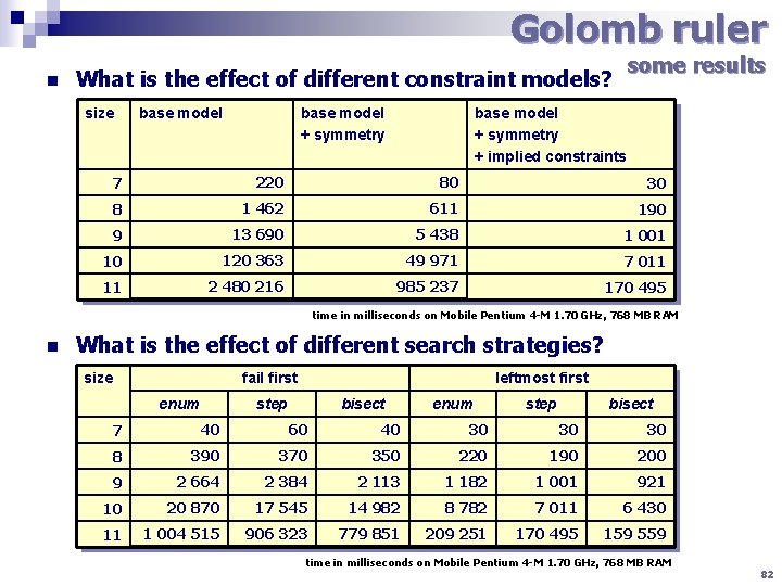
Golomb ruler n some results What is the effect of different constraint models? size base model + symmetry + implied constraints 7 220 80 30 8 1 462 611 190 9 13 690 5 438 1 001 10 120 363 49 971 7 011 11 2 480 216 985 237 170 495 time in milliseconds on Mobile Pentium 4 -M 1. 70 GHz, 768 MB RAM n What is the effect of different search strategies? size fail first enum leftmost first step bisect enum step bisect 7 40 60 40 30 30 30 8 390 370 350 220 190 200 9 2 664 2 384 2 113 1 182 1 001 921 10 20 870 17 545 14 982 8 782 7 011 6 430 11 1 004 515 906 323 779 851 209 251 170 495 159 559 time in milliseconds on Mobile Pentium 4 -M 1. 70 GHz, 768 MB RAM 82

Conclusions

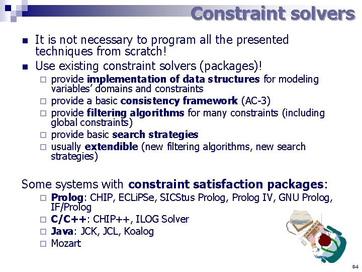
Constraint solvers n n It is not necessary to program all the presented techniques from scratch! Use existing constraint solvers (packages)! ¨ ¨ ¨ provide implementation of data structures for modeling variables’ domains and constraints provide a basic consistency framework (AC-3) provide filtering algorithms for many constraints (including global constraints) provide basic search strategies usually extendible (new filtering algorithms, new search strategies) Some systems with constraint satisfaction packages: Prolog: CHIP, ECLi. PSe, SICStus Prolog, Prolog IV, GNU Prolog, IF/Prolog ¨ C/C++: CHIP++, ILOG Solver ¨ Java: JCK, JCL, Koalog ¨ Mozart ¨ 84

n Books ¨ ¨ ¨ n P. Van Hentenryck: Constraint Satisfaction in Logic Programming, MIT Press, 1989 E. Tsang: Foundations of Constraint Satisfaction, Academic Press, 1993 K. Marriott, P. J. Stuckey: Programming with Constraints: An Introduction, MIT Press, 1998 T. Frühwirth, S. Abdennadher: Essentials of Constraint Programming, Springer Verlag, 2003 R. Dechter: Constraint Processing, Morgan Kaufmann, 2003 Journal ¨ n Resources Constraints, An International Journal. Kluwer Academic Publishers (Springer) On-line materials ¨ On-line Guide to Constraint Programming (tutorial) http: //kti. mff. cuni. cz/~bartak/constraints/ ¨ Constraints Archive (archive and links) http: //4 c. ucc. ie/web/archive/index. jsp ¨ Constraint Programming online (community web) http: //www. cp-online. org/ 85

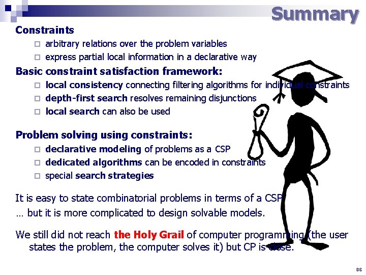
Constraints Summary arbitrary relations over the problem variables ¨ express partial local information in a declarative way ¨ Basic constraint satisfaction framework: local consistency connecting filtering algorithms for individual constraints ¨ depth-first search resolves remaining disjunctions ¨ local search can also be used ¨ Problem solving using constraints: declarative modeling of problems as a CSP ¨ dedicated algorithms can be encoded in constraints ¨ special search strategies ¨ It is easy to state combinatorial problems in terms of a CSP … but it is more complicated to design solvable models. We still did not reach the Holy Grail of computer programming (the user states the problem, the computer solves it) but CP is close. 86