Constant Temperature Anemometry A Theoretical Introduction by Dr

Constant Temperature Anemometry A Theoretical Introduction, by Dr. F. Gökhan Ergin

Purpose and aim › Purpose: to measure mean and fluctuating velocity components in fluid flows › Aim of slide show: −to explain how Constant Temperature Anemometry (CTA) can be used for this purpose −serve as education material for undergraduate and graduate courses in experimental fluid mechanics 11/26/2020 Copyright © 2016. Dantec Dynamics. All rights reserved 2

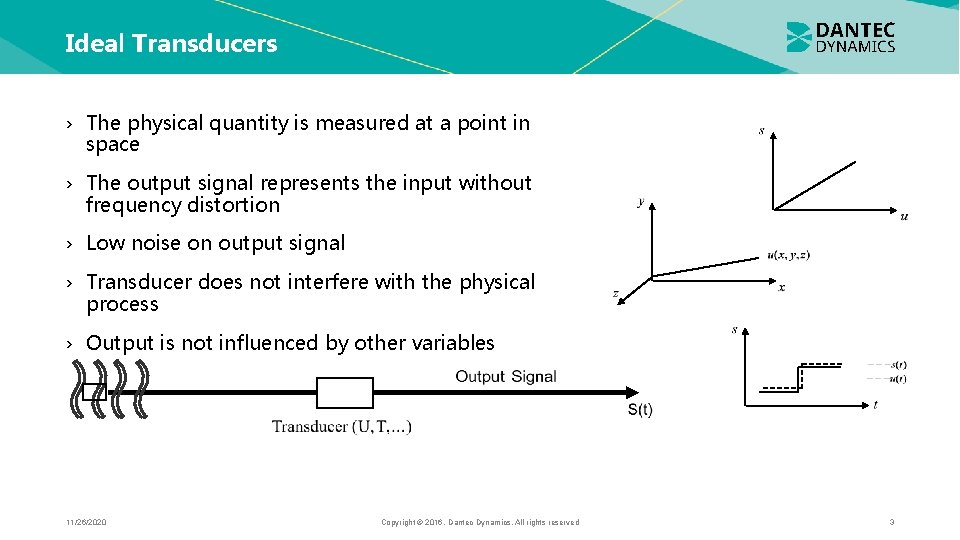
Ideal Transducers › The physical quantity is measured at a point in space › The output signal represents the input without frequency distortion › Low noise on output signal › Transducer does not interfere with the physical process › Output is not influenced by other variables 11/26/2020 Copyright © 2016. Dantec Dynamics. All rights reserved 3

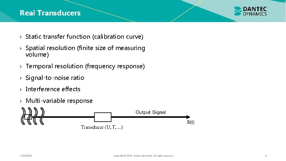
Real Transducers › Static transfer function (calibration curve) › Spatial resolution (finite size of measuring volume) › Temporal resolution (frequency response) › Signal-to-noise ratio › Interference effects › Multi-variable response 11/26/2020 Copyright © 2016. Dantec Dynamics. All rights reserved 4

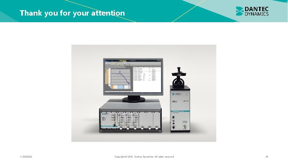
State of the art CTA system Stream. Line Pro system with automatic probe calibrator

Operation principle › Consider a thin wire mounted to supports and exposed to a velocity U. › When a current is passed through wire, heat is generated (I 2 Rw). In equilibrium, this must be balanced by heat loss (primarily convective) to the surroundings. › If velocity changes, convective heat transfer coefficient will change, wire temperature will change and eventually reach a new equilibrium. 11/26/2020 Copyright © 2016. Dantec Dynamics. All rights reserved 6

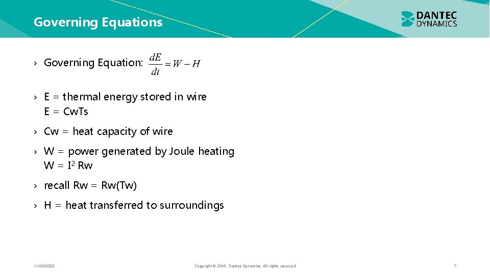
Governing Equations › Governing Equation: › E = thermal energy stored in wire E = Cw. Ts › Cw = heat capacity of wire › W = power generated by Joule heating W = I 2 Rw › recall Rw = Rw(Tw) › H = heat transferred to surroundings 11/26/2020 Copyright © 2016. Dantec Dynamics. All rights reserved 7

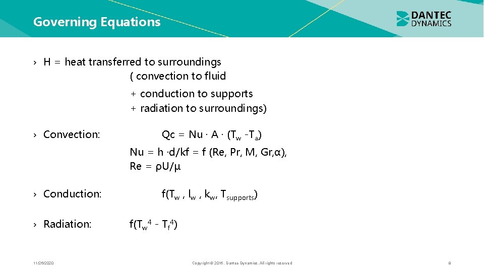
Governing Equations › H = heat transferred to surroundings ( convection to fluid + conduction to supports + radiation to surroundings) › Convection: Qc = Nu · A · (Tw -Ta) Nu = h ·d/kf = f (Re, Pr, M, Gr, α), Re = ρU/µ › Conduction: › Radiation: 11/26/2020 f(Tw , lw , kw, Tsupports) f(Tw 4 - Tf 4) Copyright © 2016. Dantec Dynamics. All rights reserved 8

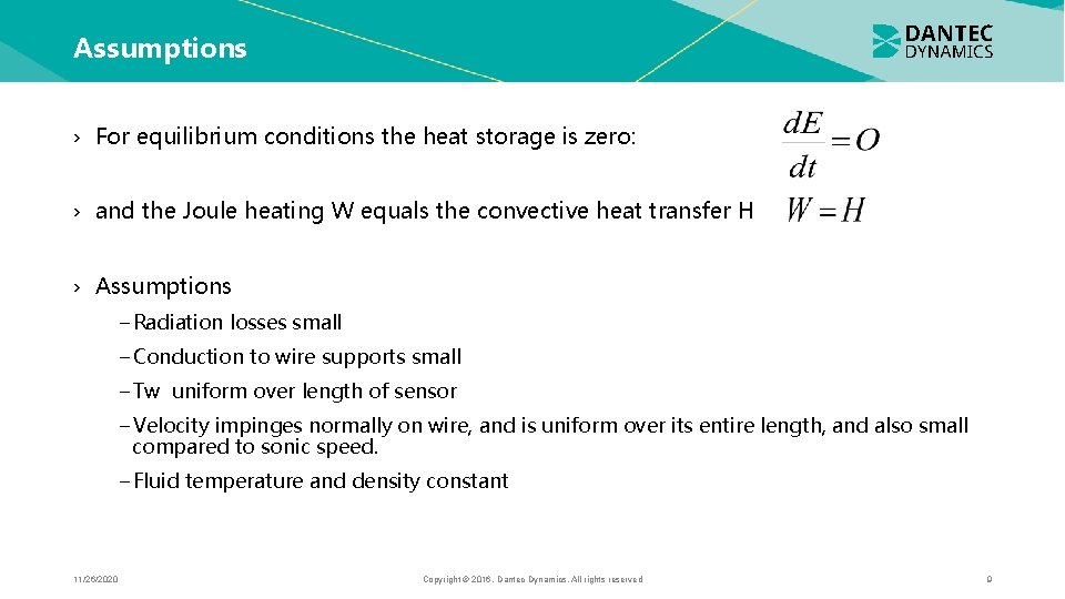
Assumptions › For equilibrium conditions the heat storage is zero: › and the Joule heating W equals the convective heat transfer H › Assumptions −Radiation losses small −Conduction to wire supports small −Tw uniform over length of sensor −Velocity impinges normally on wire, and is uniform over its entire length, and also small compared to sonic speed. −Fluid temperature and density constant 11/26/2020 Copyright © 2016. Dantec Dynamics. All rights reserved 9

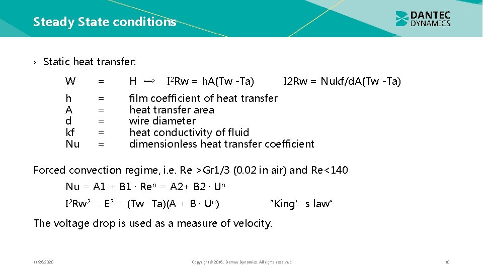
Steady State conditions › Static heat transfer: W = H I 2 Rw = h. A(Tw -Ta) I 2 Rw = Nukf/d. A(Tw -Ta) h A d kf Nu = = = film coefficient of heat transfer area wire diameter heat conductivity of fluid dimensionless heat transfer coefficient Forced convection regime, i. e. Re >Gr 1/3 (0. 02 in air) and Re<140 Nu = A 1 + B 1 · Ren = A 2+ B 2 · Un I 2 Rw 2 = E 2 = (Tw -Ta)(A + B · Un) “King’s law” The voltage drop is used as a measure of velocity. 11/26/2020 Copyright © 2016. Dantec Dynamics. All rights reserved 10

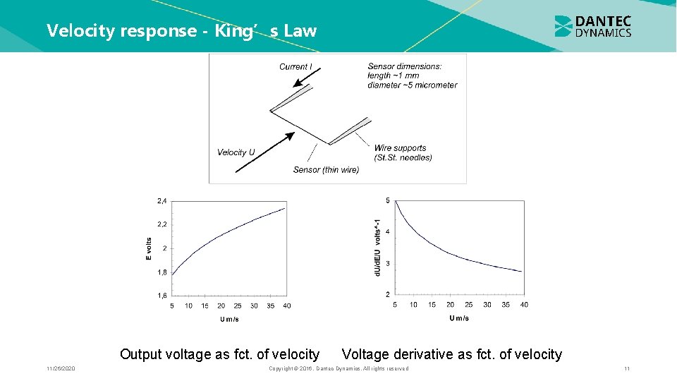
Velocity response - King’s Law Output voltage as fct. of velocity 11/26/2020 Voltage derivative

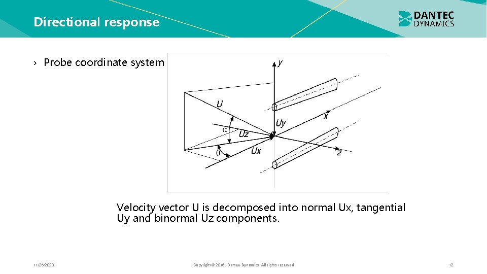
Directional response › Probe coordinate system Velocity vector U is decomposed into normal Ux, tangential Uy and binormal Uz components. 11/26/2020 Copyright © 2016. Dantec Dynamics. All rights reserved 12

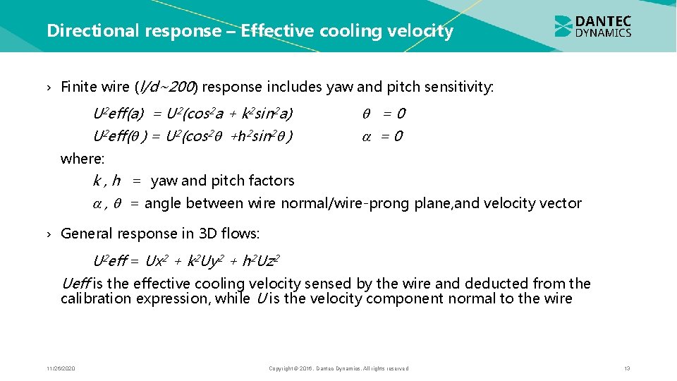
Directional response – Effective cooling velocity › Finite wire (l/d~200) response includes yaw and pitch sensitivity: U 2 eff(a) = U 2(cos 2 a + k 2 sin 2 a) U 2 eff( ) = U 2(cos 2 +h 2 sin 2 ) =0 where: k , h = yaw and pitch factors , = angle between wire normal/wire-prong plane, and velocity vector › General response in 3 D flows: U 2 eff = Ux 2 + k 2 Uy 2 + h 2 Uz 2 Ueff is the effective cooling velocity sensed by the wire and deducted from the calibration expression, while U is the velocity component normal to the wire 11/26/2020 Copyright © 2016. Dantec Dynamics. All rights reserved 13

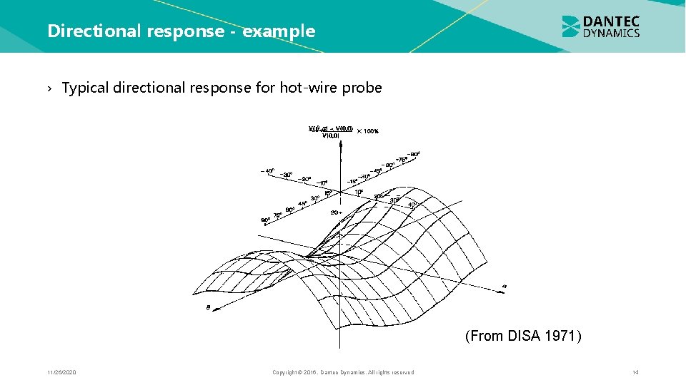
Directional response - example › Typical directional response for hot-wire probe (From DISA 1971)

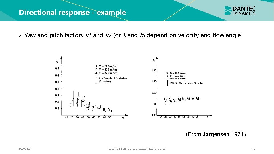
Directional response - example › Yaw and pitch factors k 1 and k 2 (or k and h) depend on velocity and flow angle (From Jørgensen 1971) 11/26/2020 Copyright © 2016. Dantec Dynamics. All rights reserved 15

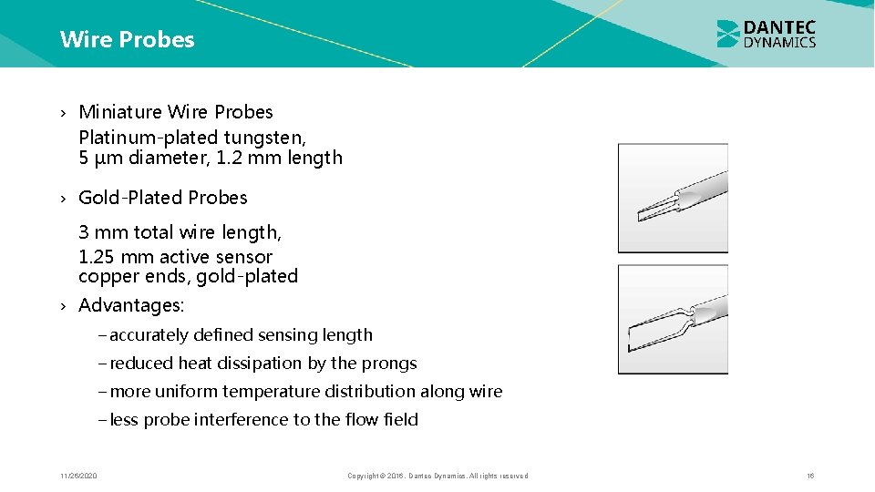
Wire Probes › Miniature Wire Probes Platinum-plated tungsten, 5 µm diameter, 1. 2 mm length › Gold-Plated Probes 3 mm total wire length, 1. 25 mm active sensor copper ends, gold-plated › Advantages: −accurately defined sensing length −reduced heat dissipation by the prongs −more uniform temperature distribution along wire −less probe interference to the flow field 11/26/2020 Copyright © 2016. Dantec Dynamics. All rights reserved 16

Wire Probes › For optimal frequency response, the probe should have as small a thermal inertia as possible. Important considerations: › Wire length should be as short as possible (spatial resolution; want probe length << eddy size) › Aspect ratio (l/d) should be high (to minimize effects of end losses) › Wire should resist oxidation until high temperatures (want to operate wire at high T to get good sensitivity, high signal to noise ratio) › Temperature coefficient of resistance should be high (for high sensitivity, signal to noise ratio and frequency response) › Wires of less than 5 µm diameter cannot be drawn with reliable diameters 11/26/2020 Copyright © 2016. Dantec Dynamics. All rights reserved 17

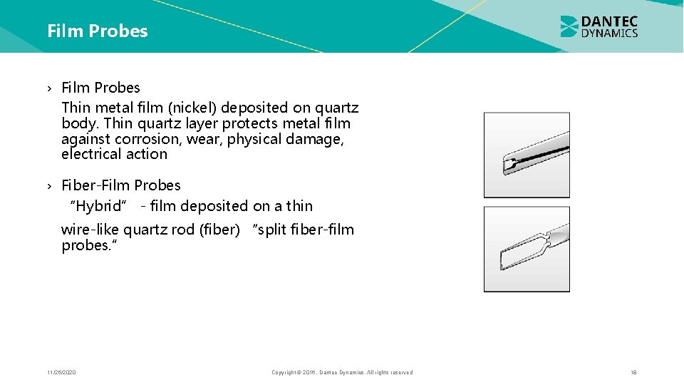
Film Probes › Film Probes Thin metal film (nickel) deposited on quartz body. Thin quartz layer protects metal film against corrosion, wear, physical damage, electrical action › Fiber-Film Probes “Hybrid” - film deposited on a thin wire-like quartz rod (fiber) “split fiber-film probes. ” 11/26/2020 Copyright © 2016. Dantec Dynamics. All rights reserved 18

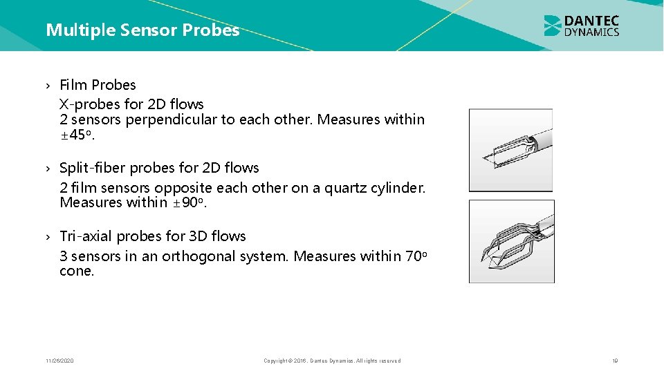
Multiple Sensor Probes › Film Probes X-probes for 2 D flows 2 sensors perpendicular to each other. Measures within ± 45 o. › Split-fiber probes for 2 D flows 2 film sensors opposite each other on a quartz cylinder. Measures within ± 90 o. › Tri-axial probes for 3 D flows 3 sensors in an orthogonal system. Measures within 70 o cone. 11/26/2020 Copyright © 2016. Dantec Dynamics. All rights reserved 19

Probe Selection › Use wire probes whenever possible - relatively inexpensive - better frequency response - can be repaired › Use film probes for rough environments - more rugged - worse frequency response - cannot be repaired - electrically insulated - protected against mechanical and chemical action 11/26/2020 Copyright © 2016. Dantec Dynamics. All rights reserved 20

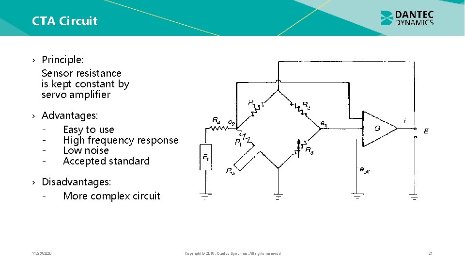
CTA Circuit › Principle: Sensor resistance is kept constant by servo amplifier › Advantages: Easy to use High frequency response Low noise Accepted standard › Disadvantages: More complex circuit 11/26/2020 Copyright © 2016. Dantec Dynamics. All rights reserved 21

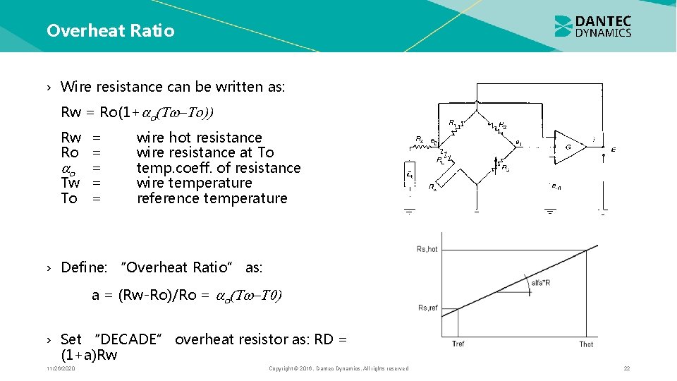
Overheat Ratio › Wire resistance can be written as: Rw = Ro(1+ Rw = Ro = = Tw = To = wire hot resistance wire resistance at To temp. coeff. of resistance wire temperature reference temperature › Define: “Overheat Ratio” as: a = (Rw-Ro)/Ro = › Set “DECADE” overheat resistor as: RD = (1+a)Rw 11/26/2020 Copyright © 2016. Dantec Dynamics. All rights reserved 22

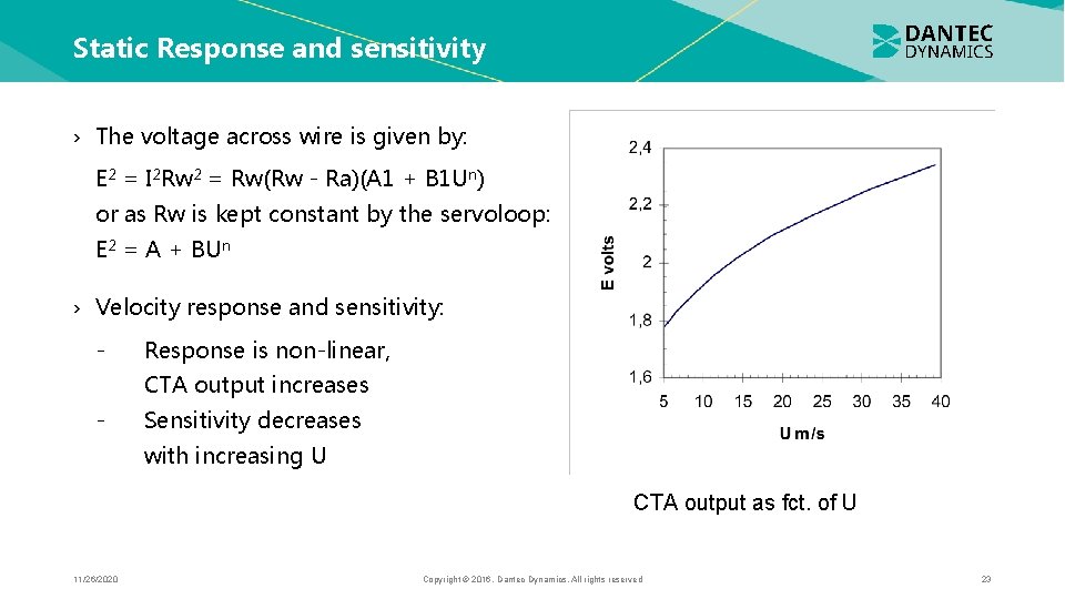
Static Response and sensitivity › The voltage across wire is given by: E 2 = I 2 Rw 2 = Rw(Rw - Ra)(A 1 + B 1 Un) or as Rw is kept constant by the servoloop: E 2 = A + BUn › Velocity response and sensitivity: - Response is non-linear, CTA output increases - Sensitivity decreases with increasing U CTA output as fct. of U 11/26/2020 Copyright © 2016. Dantec Dynamics. All rights reserved 23

Static Response to velocity › Despite extensive work, no universal expression to describe heat transfer from hot wires and films exist. › For all actual measurements, direct calibration of the anemometer system against a well-known velocity reference is necessary. 11/26/2020 Copyright © 2016. Dantec Dynamics. All rights reserved 24

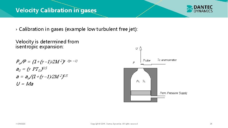
Velocity Calibration in gases › Calibration in gases (example low turbulent free jet): Velocity is determined from isentropic expansion: Po/P = (1+( 2) a 0 = ( 0 )0. 5 a = ao/(1+( 2)0. 5 U = Ma 11/26/2020 Copyright © 2016. Dantec Dynamics. All rights reserved 25

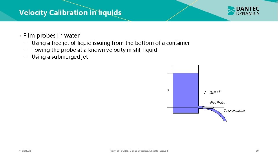
Velocity Calibration in liquids › Film probes in water − Using a free jet of liquid issuing from the bottom of a container − Towing the probe at a known velocity in still liquid − Using a submerged jet 11/26/2020 Copyright © 2016. Dantec Dynamics. All rights reserved 26

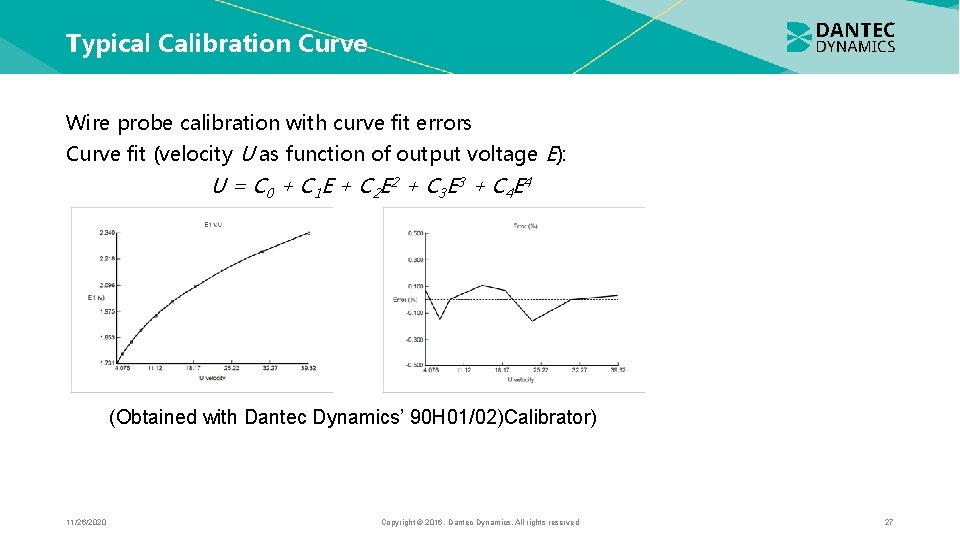
Typical Calibration Curve Wire probe calibration with curve fit errors Curve fit (velocity U as function of output voltage E): U = C 0 + C 1 E + C 2 E 2 + C 3 E 3 + C 4 E 4 (Obtained with Dantec Dynamics’ 90 H 01/02)Calibrator) 11/26/2020 Copyright © 2016. Dantec Dynamics. All rights reserved 27

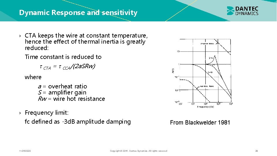
Dynamic Response and sensitivity › CTA keeps the wire at constant temperature, hence the effect of thermal inertia is greatly reduced: Time constant is reduced to CTA = CCA/(2 a. SRw) where a = overheat ratio S = amplifier gain Rw = wire hot resistance › Frequency limit: fc defined as -3 d. B amplitude damping 11/26/2020 Copyright © 2016. Dantec Dynamics. All rights reserved From Blackwelder 1981 28

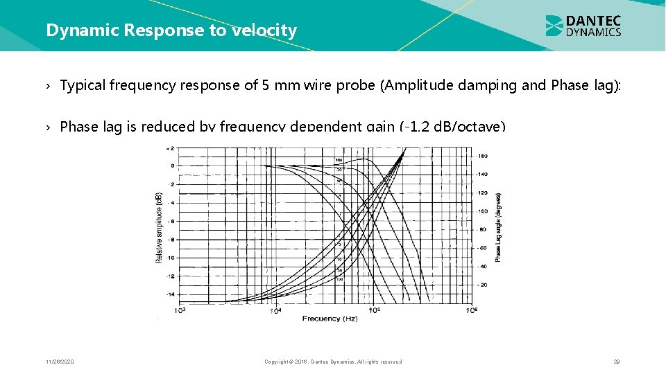
Dynamic Response to velocity › Typical frequency response of 5 mm wire probe (Amplitude damping and Phase lag): › Phase lag is reduced by frequency dependent gain (-1. 2 d. B/octave) 11/26/2020 Copyright © 2016. Dantec Dynamics. All rights reserved 29

Dynamic Calibration – Direct Method › Need a flow in which sinusoidal velocity variations of known amplitude are superimposed on a constant mean velocity − Microwave simulation of turbulence (<500 Hz) − Sound field simulation of turbulence (>500 Hz) − Vibrating the probe in a laminar flow (<1000 Hz) All methods are difficult and are restricted to low frequencies. 11/26/2020 Copyright © 2016. Dantec Dynamics. All rights reserved 30

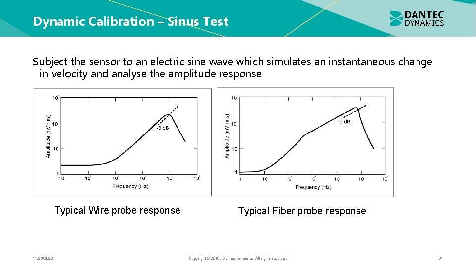
Dynamic Calibration – Sinus Test Subject the sensor to an electric sine wave which simulates an instantaneous change in velocity and analyse the amplitude response Typical Wire probe response 11/26/2020 Typical Fiber probe response Copyright © 2016. Dantec Dynamics. All rights reserved 31

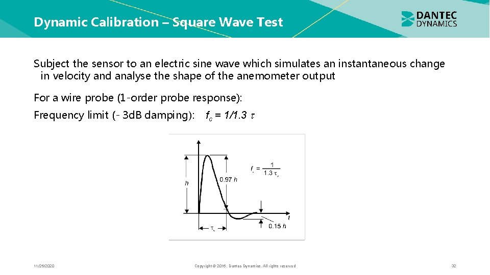
Dynamic Calibration – Square Wave Test Subject the sensor to an electric sine wave which simulates an instantaneous change in velocity and analyse the shape of the anemometer output For a wire probe (1 -order probe response): Frequency limit (- 3 d. B damping): 11/26/2020 fc = 1/1. 3 Copyright © 2016. Dantec Dynamics. All rights reserved 32

Dynamic Calibration – Conclusions › Indirect methods are the only ones applicable in practice. › Sinus test necessary for determination of frequency limit for fiber and film probes. › Square wave test determines frequency limits for wire probes. Time taken by the anemometer to rebalance itself is used as a measure of its frequency response. › Square wave test is primarily used for checking dynamic stability of CTA at high velocities. › Indirect methods cannot simulate effect of thermal boundary layers around sensor (which reduces the frequency response). 11/26/2020 Copyright © 2016. Dantec Dynamics. All rights reserved 33

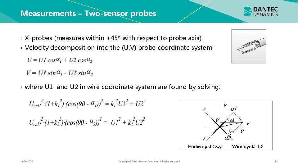
Measurements – Two-sensor probes › X-probes (measures within ± 45 o with respect to probe axis): › Velocity decomposition into the (U, V) probe coordinate system › where U 1 and U 2 in wire coordinate system are found by solving: 11/26/2020 Copyright © 2016. Dantec Dynamics. All rights reserved 34

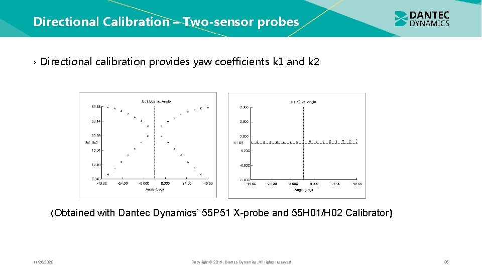
Directional Calibration – Two-sensor probes › Directional calibration provides yaw coefficients k 1 and k 2 (Obtained with Dantec Dynamics’ 55 P 51 X-probe and 55 H 01/H 02 Calibrator) 11/26/2020 Copyright © 2016. Dantec Dynamics. All rights reserved 35

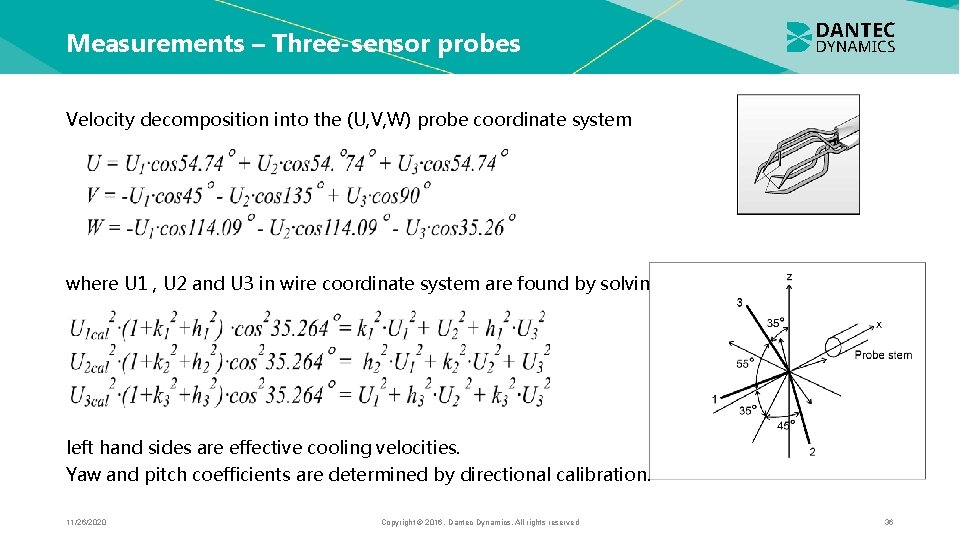
Measurements – Three-sensor probes Velocity decomposition into the (U, V, W) probe coordinate system where U 1 , U 2 and U 3 in wire coordinate system are found by solving: left hand sides are effective cooling velocities. Yaw and pitch coefficients are determined by directional calibration. 11/26/2020 Copyright © 2016. Dantec Dynamics. All rights reserved 36

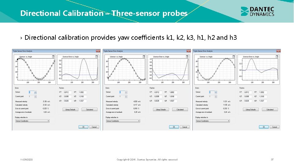
Directional Calibration – Three-sensor probes › Directional calibration provides yaw coefficients k 1, k

Uncertainty sources › Anemometer system makes use of heat transfer from the probe Qc = Nu · A · (Tw -Ta) Nu = h · d/kf = f (Re, Pr, M, Gr, › Anything which changes this heat transfer (other than the flow variable being measured) is an Uncertainly Source › Unsystematic effects (contamination, air bubbles in water, probe vibrations, etc. ) › Systematic effects (ambient temperature variations, solid wall proximity, eddy shedding from cylindrical sensors etc. ) 11/26/2020 Copyright © 2016. Dantec Dynamics. All rights reserved 38

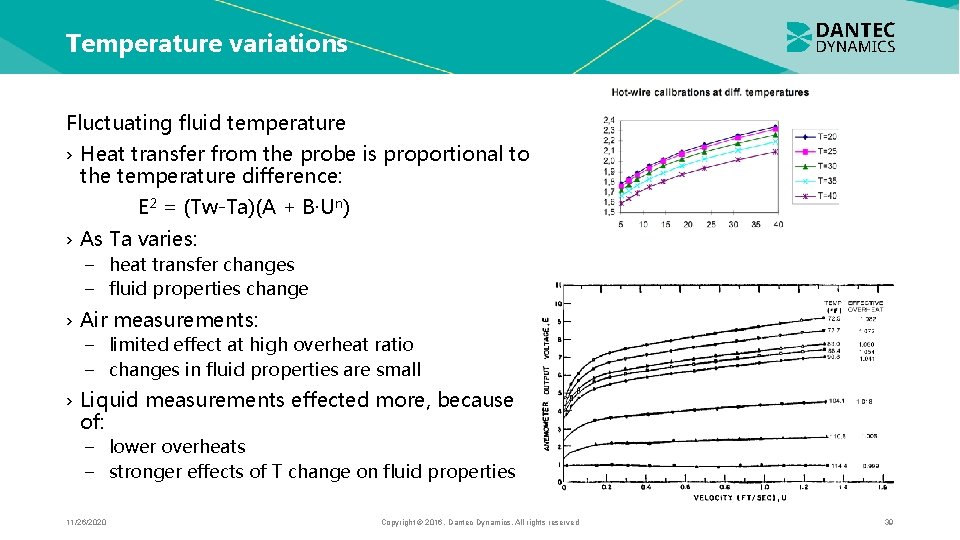
Temperature variations Fluctuating fluid temperature › Heat transfer from the probe is proportional to the temperature difference: E 2 = (Tw-Ta)(A + B·Un) › As Ta varies: − heat transfer changes − fluid properties change › Air measurements: − limited effect at high overheat ratio − changes in fluid properties are small › Liquid measurements effected more, because of: − lower overheats − stronger effects of T change on fluid properties 11/26/2020 Copyright © 2016. Dantec Dynamics. All rights reserved 39

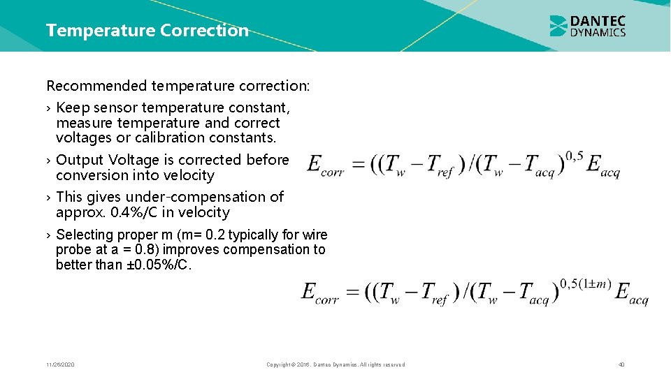
Temperature Correction Recommended temperature correction: › Keep sensor temperature constant, measure temperature and correct voltages or calibration constants. › Output Voltage is corrected before conversion into velocity › This gives under-compensation of approx. 0. 4%/C in velocity › Selecting proper m (m= 0. 2 typically for wire probe at a = 0. 8) improves compensation to better than ± 0. 05%/C. 11/26/2020 Copyright © 2016. Dantec Dynamics. All rights reserved 40

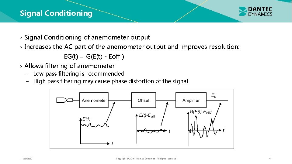
Signal Conditioning › Signal Conditioning of anemometer output › Increases the AC part of the anemometer output and improves resolution: EG(t) = G(E(t) - Eoff ) › Allows filtering of anemometer − Low pass filtering is recommended − High pass filtering may cause phase distortion of the signal 11/26/2020 Copyright © 2016. Dantec Dynamics. All rights reserved 41

Tips to get good CTA measurements › Get an idea of the flow (velocity range, dimensions, frequency) › Select right probe and anemometer configuration › Select proper A/D board › Perform set-up (hardware set-up, velocity calibration, directional calibration) › Make a first rough verification of the assumptions about the flow › Define experiment (traverse, sampling frequency, Nyquist and number of samples) › Perform the experiment › Reduce the data (moments, spectra, correlations) › Evaluate results › Recalibrate to make sure that the anemometer/probe has not drifted 11/26/2020 Copyright © 2016. Dantec Dynamics. All rights reserved 42