CONIFUNNELING Stringy tunneling between flux vacua David Kagan

CONIFUNNELING Stringy tunneling between flux vacua David Kagan Columbia University, ISCAP Work in progress (to appear soon) with Brian Greene, Eugene Lim, Saswat Sarangi, I-Sheng Yang, and Pontus Ahlqvist

Motivation

Motivation

Motivation String theory is the best candidate for a theory of quantum gravity. As such, it should have important things to tell us about the very early universe. Furthermore, going from 10 D to 4 D leads to a very rich vacuum structure whose connectivity is an interesting topic in its own right. Having multitudes of vacua should have bearing on scenarios like eternal inflation, where bubble universes sample the possible vacua. Master plan: build a model of a stringy, inflating universe.

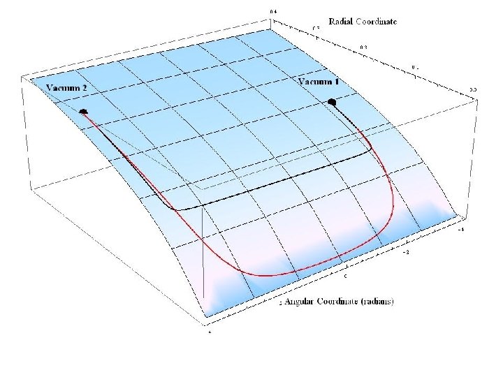
CONIFUNNELING: What is it? Tunneling paths between certain flux vacua appear to be driven very close to the conifold point in a Calabi-Yau’s complex moduli space

CONIFUNNELING: What is it? Tunneling paths between certain flux vacua appear to be driven very close to the conifold point in a Calabi-Yau’s complex moduli space Physically, the path represents nucleation of a 5 -brane. It makes sense that such a process “prefers” to occur when the brane can wrap a small cycle.

CONIFUNNELING: What is it? We should expect similar behavior for other types of brane-mediated processes. The energetics should be a competition between changing cycles and nucleating branes with appropriate charges. This should have implications for how one transits between different flux vacua in a network of such vacua (as modeled for instance by Bousso and Polchinski)

CONIFUNNELING: What is it? Finally, if—as we shall see—the wrapped cycles get very small, we should expect warping to play an essential role in the dynamics. Incorporating warping is hard! We will do so at a relatively qualitative level that I will describe later. Previous studies of field dynamics along the lines of our approach: [ar. Xiv/0805. 3705]

Basic set-up Work with type IIB stringµtheory in the supergravity¶limit: R p 2 F~ 2 j. G( 3) j 2 ¿j j 1 10 = SI I B ¡ ¡ ( 5 ) + SC S + Sl oc d x ¡ g R¡ 2· with SCS = 1 8 i · 210 12¿I 2¿ 2 2 10 I RC ( 4) 4¢ 5! ^ G( 3) ¿I And compactify on a Calabi-Yau, so take M 10 » M 4 £ CY 6

Basic set-up: Calabi-Yau Despite not having explicit metrics, compact CY’s are very special manifolds. Their properties can be used to deduce the information relevant for the 4 D effective theory. In particular, deformations of the metric are highly constrained. ¢ gz z¹ ¢ gzz

Basic set-up: Calabi-Yau M odel ® ® # 1 2 3 4 5 6 7 8 9 10 11 12 13 14 P 4 [5] WP 2; 1; 1 [6] WP 4; 1; 1 [8] WP 5; 2; 1; 1; 1 [10] WP 2; 1; 1; 1 [3; 4] WP 3; 2; 2; 1; 1; 1 [4; 6] * P 5 [2; 4] P 6 [2; 2; 3] WP 3; 1; 1; 1 [2; 6] P 5 [3; 3] WP 2; 2; 1; 1 [4; 4] WP 3; 3; 2; 2; 1; 1 [6; 6] P 7 [2; 2; 2; 2] 1 2 3 1=5 1=6 1=8 1=10 1=4 1=6 1=12 1=4 1=3 1=6 1=3 1=4 1=6 1=2 2=5 1=3 3=8 3=10 1=3 1=4 5=12 1=2 1=3 1=4 1=6 1=2 3=5 2=3 5=8 7=10 2=3 3=4 7=12 1=2 1=2 2=3 3=4 5=6 1=2 4 4=5 5=6 7=8 9=10 3=4 5=6 11=12 3=4 2=3 5=6 2=3 3=4 5=6 1=2 m 1 -4 -3 -3 -2 -4 -2 -3 -5 -6 -4 -5 -3 -1 -7 m 2 5 4 4 3 5 3 4 6 7 5 6 4 2 8 m 3 -5 -3 -2 -1 -6 -2 -1 -8 -12 -4 -9 -4 -1 -16 m 4 5 3 2 1 6 2 1 8 12 4 9 4 1 16 We look at the 14 models with only one complex structure modulus to start with (most computationally tractable – ignore Kahler moduli stabilization!).

Basic set-up: Calabi-Yau Periods With one complex modulus, a Calabi-Yau manifold has four nontrivial 3 -cycles 0 around 1 which can be defined periods ¦ B¦ ¦ (z) = B @¦ ¦ 3 (z) C (z) 2 C A (z) 1 0 (z)

Basic set-up: Calabi-Yau Periods These periods are not single-valued functions on the moduli space. Around the special points z = 0; 1; 1 the periods transform by 0 1 a monodromy 0 ¦ B¦ B @¦ ¦ ¦ C B¦ (z) 2 C ¡ ! T ¢B A @¦ (z) 1 ¦ 0 (z) 3 (z) 1 C (z) 2 C A (z) 1 0 (z)

Basic set-up: Calabi-Yau Periods For example, monodromy around the conifold point z= 1 yields 0 1 ¦ 3 (z) B ¦ (z) C B 2 C ¡! @¦ (z) A 1 ¦ 0 (z) 0 1 B 0 B @0 1 0 0 C C 0 A 1 0 ¦ B¦ B @¦ ¦ 3 (z) 1 0 C B = B A @ (z) 1 ¦ 0 (z) 2 (z) C 1 ¦ 3 (z) C ¦ 2 (z) C A ¦ 1 (z) 0 (z) + ¦ 3 (z)

Im(z) K z z¹ Re(z) The Kahler metric: field space has non-trivial geometry

1 j zj 2 Im(z) Origin is the LCS point K z z¹ Re(z) The Kahler metric: field space has non-trivial geometry

Log divergence from special geometry Im(z) z= 1 K z z¹ Re(z) The Kahler metric: field space has non-trivial geometry

Fluxes off, Potential trivial

Fluxes switched on…

Turning on Fluxes The NS-NS and R-R 3 -form field strengths can provide fluxes that pierce the various 3 -cycles. This generates a superpotential W = (F ¡ ¿H ) ¢¦ (z) 0 1 F 0 BF C 1 C F = B @F A 2 F 3 0 1 H 0 BH C 1 C H = B @H A 2 H 3

Turning on Fluxes Assume Kahler moduli are stabilized somehow (KKLT perhaps). At tree level, cancellations occur between Kahler modulus terms and a negative-definite term in the flux potential. ¡ So at tree level we are left with the no-scale flux potential V = e. K K z z¹ j. D z W j 2 + K ¿¿¹ j. D ¿ W j 2 ¢

Fluxes versus Monodromy The superpotential is indifferent about whether we transform periods versus flux vectors W = (F ¡ ¿H ) ¢¦ (z) 0 1 F 0 BF C B 1 C @F A 2 F 3 0 > ¡! 1 F 0 BF C B 1 C @F A 2 F 3 > 0 1 B 0 ¢B @0 1 0 0 (and similarly for NS-NS fluxes H) 0 0 1 0 1> 0 F 0 + F 3 B F C 0 C 1 C = B C @ F A 0 A 2 1 F 3

Vacuum Hunting We explore flux potential “topography” [see ar. Xiv, hep-th/061222] Finding vacua is not easy! Have to essentially guess at a correct combination of fluxes.

Vacuum Hunting: Analog Vacua

Vacuum Hunting: Analog Vacua

Vacuum Hunting: Analog Vacua

Chains of SUSY vacua for different one-parameter Calabi-Yau compactifications. Round dots are the locations of SUSY flux vacua for different (connected) fluxes Dz. W = 0 D ¿W = 0

Finding the domain wall Tunneling is multi-field – hard to just guess the right path Non-standard kinetic terms complicate matters as well.

Finding the domain wall h @ G ij @t i @Ái @t = ¡ ¡ h @ G ij @x @V @Áj + i @Ái @x 1 @G k l 2 @Áj h @Ák @Ál @t @t ¡ i @Ák @Ál @x @x

Finding the domain wall h @ G ij @t i @Ái @t = ¡ ¡ h @ G ij @x @V @Áj + i @Ái @x 1 @G k l 2 @Áj h @Ák @Ál @t @t ¡ i @Ák @Ál @x @x Mmm…relax you must to find correct path

A simple example @2 Á @t 2 ¡ @2 Á @x 2 = ¡ @V @Á

In the bulk of the moduli space our guesses… …relax toward the conifold point

We can try to see what the possibilities are for a solution passing close to the conifold… Toy Lagrangian Two vacua in a plane with no cuts

Clearly the natural tunneling path should be a straight line.

The radial profile The angular profile Note: the angle that is turned through is just π

Now consider a two sheeted potential with vacua separated by a branch cut on the zplane.

Now consider a two sheeted potential with vacua separated by a branch cut on the zplane. The solution connecting these 2¼will want to essentially make a rotation through an angle of. This will not be possible.

Modify the model with a non-trivial kinetic term: Make a redefinition of the radial field In terms of this field we have So the maximal angle becomes

Modify the model with a non-trivial kinetic term: Make a redefinition of the radial field In terms of this field we have So the maximal angle becomes We thus need r¡ K (r ) = at least 1

Log divergence from special geometry Im(z) z= 1 K z z¹ Re(z) Special geometry implies the Kahler metric diverges as a logarithm at the conifold point, but…

As the complex modulus field approaches the conifold point, warping starts to matter. The Kahler metric is corrected: K z z¹ » ¡ log r + C r 4=3

The parametric dependence on the modulus is even better than the minimum exponent we required from before! K z z¹ » ¡ log r + C r 4=3

The new term is suppressed by the large volume of the Calabi. Yau. Only kicks in when we’re very close. K z z¹ » ¡ log r + We use an expression arising from studies by Douglas and Torroba [ar. Xiv/0805. 3700]. This is likely WRONG but parametrically okay. Qualitatively speaking, the parametric dependence on the collapsing modulus is all we need. For more discussion see Chen, Nakayama, Shiu [ar. Xiv/0905. 4463]. C r 4=3

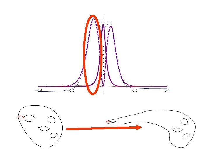
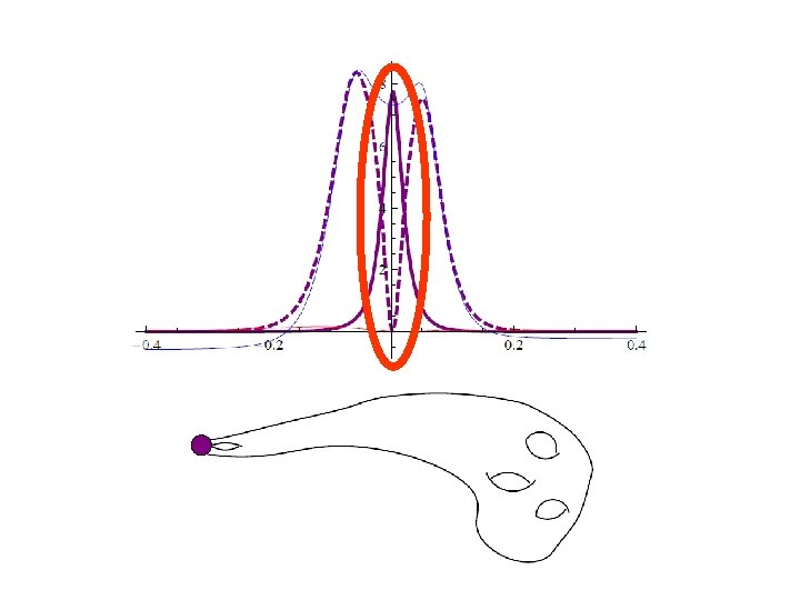
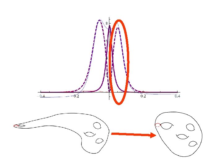
Near the conifold

Angular coordinate near the conifold (blue is the relaxed solution)

Radial coordinate near the conifold (blue is the relaxed solution)

Contributions to the action split up: Thin blue – potential Dotted – radial Solid – angle Other - ¿I ; R

CONIFUNNELING: Summary • Hunted for flux vacua in various Calabi-Yau compactifications using trial-and-error. Uncovered some patterns. • Studied transitions between V = 0 vacua. Wrapped cycle wants to shrink a great deal before brane is nucleated.

CONIFUNNELING: What’s next? • From domain walls to tunneling solutions • Being honest about Kahler moduli • Bubble collisions in moduli space • Topological transitions • The “master plan”: simulating the early stringy universe.

CONIFUNNELING: The End! David Kagan Columbia University, ISCAP Work in progress (to appear soon) with Brian Greene, Eugene Lim, Saswat Sarangi, I-Sheng Yang, and Pontus Ahlqvist