Congestion Control Optimization Steven Low netlab CALTECH edu

Congestion Control & Optimization Steven Low netlab. CALTECH. edu Cambridge 2011

Acknowledgments Caltech: L. Chen, J. Doyle, C. Jin, G. Lee, H. Newman, A. Tang, D. Wei, B. Wydrowski, Netlab Gen 1 Uruguay: F. Paganini Swinburne: L. Andrew Princeton: M. Chiang

Goal of tutorial Top-down summary of congestion control on Internet Introduction to mathematical models of congestion control Illustration of theory-guided CC algorithm design

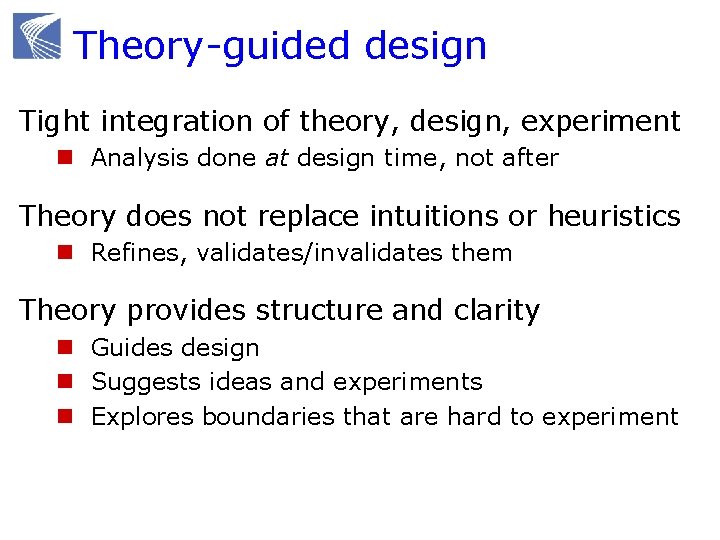
Theory-guided design Tight integration of theory, design, experiment n Analysis done at design time, not after Theory does not replace intuitions or heuristics n Refines, validates/invalidates them Theory provides structure and clarity n Guides design n Suggests ideas and experiments n Explores boundaries that are hard to experiment

Theory-guided design Integration of theory, design, experiment can be very powerful n Each needs the other n Combination much more than sum Tremendous progress in the last decade n Not as impossible as most feared n Very difficult; but worth the effort n Most critical: mindset How to push theory-guided design approach further ?

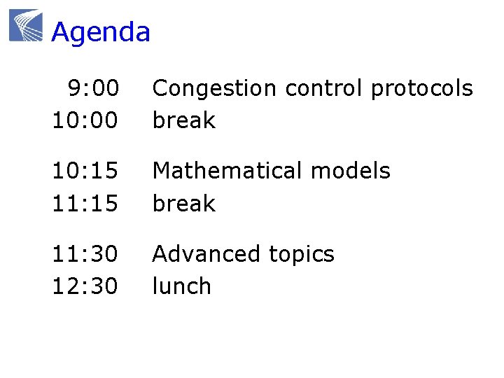
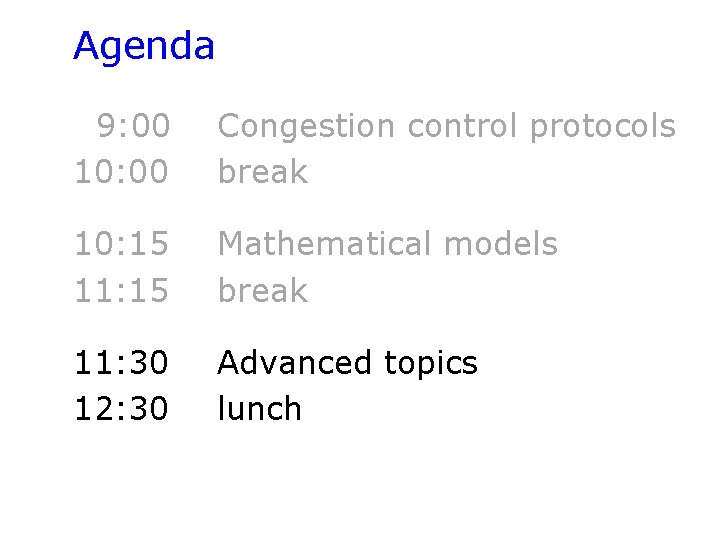
Agenda 9: 00 10: 00 Congestion control protocols break 10: 15 11: 15 Mathematical models break 11: 30 12: 30 Advanced topics lunch

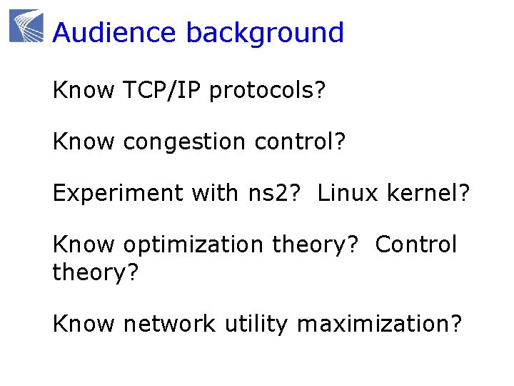
Audience background Know TCP/IP protocols? Know congestion control? Experiment with ns 2? Linux kernel? Know optimization theory? Control theory? Know network utility maximization?

CONGESTION CONTROL PROTOCOLS

Congestion control protocols Why congestion control? Where is CC implemented? Window control mechanism CC protocols and basic structure Active queue management (AQM)

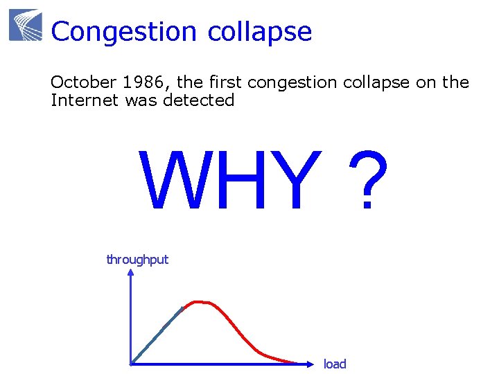
Congestion collapse October 1986, the first congestion collapse on the Internet was detected Link between UC Berkeley and LBL n 400 yards, 3 hops, 32 Kbps n throughput dropped to 40 bps n factor of ~1000 drop! WHY ? 1988, Van Jacobson proposed TCP congestion control throughput load

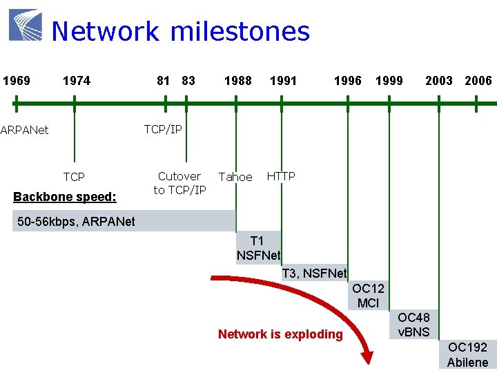
Network milestones 1969 1974 81 83 1988 1991 Tahoe HTTP 1996 1999 2003 2006 TCP/IP ARPANet TCP Backbone speed: Cutover to TCP/IP 50 -56 kbps, ARPANet T 1 NSFNet T 3, NSFNet OC 12 MCI Network is exploding OC 48 v. BNS OC 192 Abilene

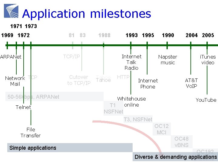
Application milestones 1971 1973 1969 1972 ARPANet Network TCP Mail 50 -56 kbps, ARPANet Telnet 81 83 TCP/IP Cutover to TCP/IP 1993 1995 1988 1990 Internet Talk Radio Tahoe HTTP 2004 2005 Napster music Internet Phone i. Tunes video AT&T Vo. IP Whitehouse online T 1 You. Tube NSFNet T 3, NSFNet File Transfer Simple applications OC 12 MCI OC 48 v. BNS OC 192 Diverse & demanding applications Abilene

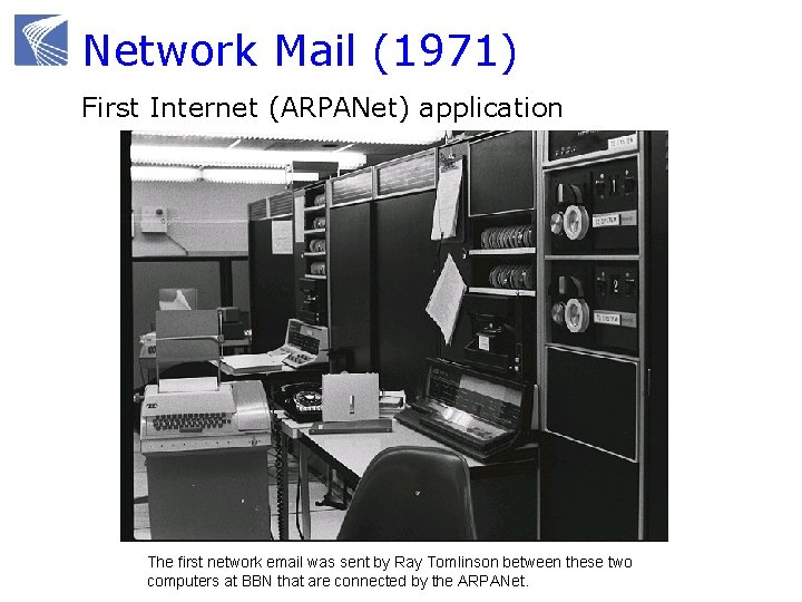
Network Mail (1971) First Internet (ARPANet) application The first network email was sent by Ray Tomlinson between these two computers at BBN that are connected by the ARPANet.

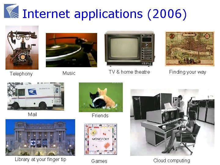
Internet applications (2006) Telephony TV & home theatre Music Mail Library at your finger tip Finding your way Friends Games Cloud computing

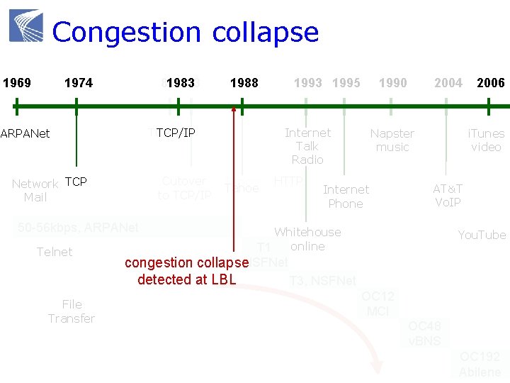
Congestion collapse 1969 1974 81 1983 83 TCP/IP ARPANet Cutover to TCP/IP Network TCP Mail 50 -56 kbps, ARPANet Telnet File Transfer 1988 1993 1995 1990 Internet Talk Radio Tahoe HTTP 2004 Napster music Internet Phone 2006 i. Tunes video AT&T Vo. IP Whitehouse online T 1 You. Tube congestion collapse. NSFNet detected at LBL T 3, NSFNet OC 12 MCI OC 48 v. BNS OC 192 Abilene

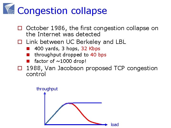
Congestion collapse o October 1986, the first congestion collapse on the Internet was detected o Link between UC Berkeley and LBL n 400 yards, 3 hops, 32 Kbps n throughput dropped to 40 bps n factor of ~1000 drop! o 1988, Van Jacobson proposed TCP congestion control throughput load

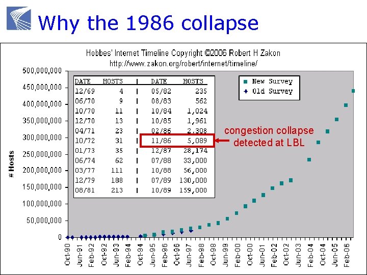
Why the 1986 collapse congestion collapse detected at LBL

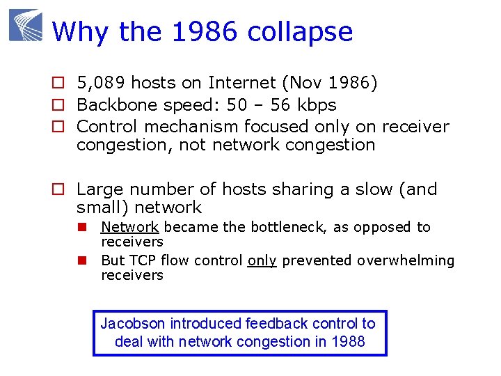
Why the 1986 collapse o 5, 089 hosts on Internet (Nov 1986) o Backbone speed: 50 – 56 kbps o Control mechanism focused only on receiver congestion, not network congestion o Large number of hosts sharing a slow (and small) network n Network became the bottleneck, as opposed to receivers n But TCP flow control only prevented overwhelming receivers Jacobson introduced feedback control to deal with network congestion in 1988

Tahoe and its variants (1988) Jacobson, Sigcomm 1988 + Avoid overwhelming network + Window control mechanisms n Dynamically adjust sender window based on congestion (as well as receiver window) n Loss-based AIMD n Based on idea of Chiu, Jain, Ramakrishnan “… important considering that TCP spans a range from 800 Mbps Cray channels to 1200 bps packet radio links” -- Jacobson, 1988

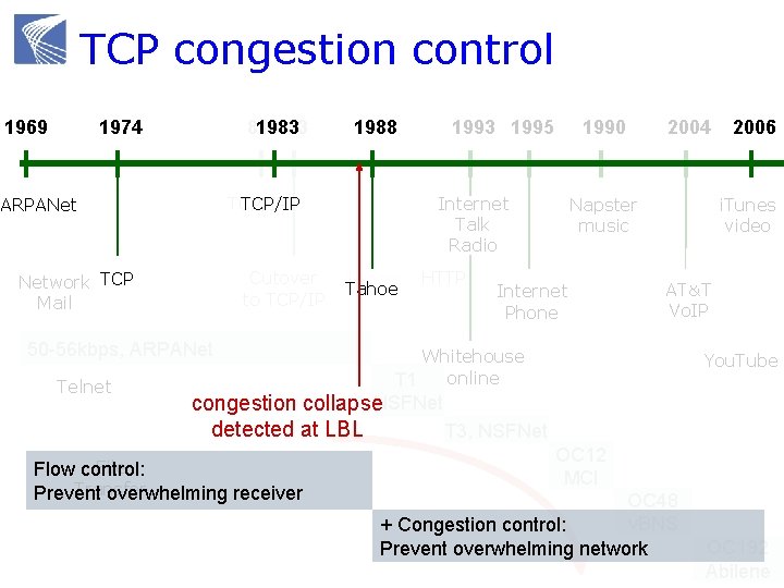
TCP congestion control 1969 1974 81 1983 83 TCP/IP ARPANet Cutover to TCP/IP Network TCP Mail 50 -56 kbps, ARPANet Telnet 1988 1993 1995 1990 Internet Talk Radio Tahoe HTTP 2004 Napster music Internet Phone 2006 i. Tunes video AT&T Vo. IP Whitehouse online T 1 You. Tube congestion collapse. NSFNet detected at LBL T 3, NSFNet File Flow control: Transfer Prevent overwhelming receiver OC 12 MCI OC 48 v. BNS + Congestion control: Prevent overwhelming network OC 192 Abilene

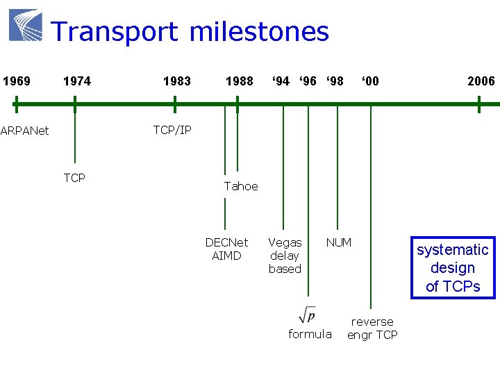
Transport milestones 1969 1974 1983 1988 ‘ 94 ‘ 96 ‘ 98 ‘ 00 2006 TCP/IP ARPANet TCP Tahoe DECNet AIMD Vegas delay based NUM formula reverse engr TCP systematic design of TCPs

Congestion control protocols Why congestion control? Where is CC implemented? Window control mechanism CC protocols and basic structure Active queue management (AQM)

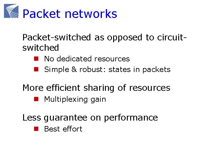
Packet networks Packet-switched as opposed to circuitswitched n No dedicated resources n Simple & robust: states in packets More efficient sharing of resources n Multiplexing gain Less guarantee on performance n Best effort

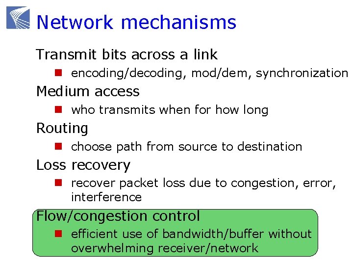
Network mechanisms Transmit bits across a link n encoding/decoding, mod/dem, synchronization Medium access n who transmits when for how long Routing n choose path from source to destination Loss recovery n recover packet loss due to congestion, error, interference Flow/congestion control n efficient use of bandwidth/buffer without overwhelming receiver/network

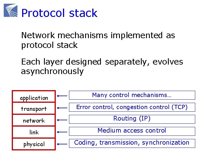
Protocol stack Network mechanisms implemented as protocol stack Each layer designed separately, evolves asynchronously application Many control mechanisms… transport Error control, congestion control (TCP) network Routing (IP) link Medium access control physical Coding, transmission, synchronization

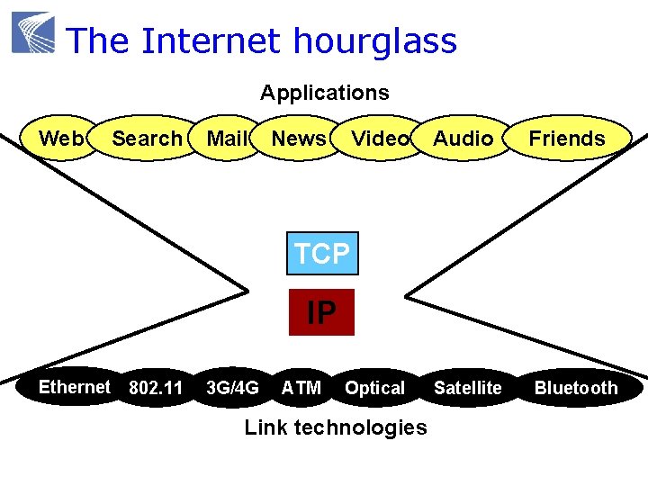
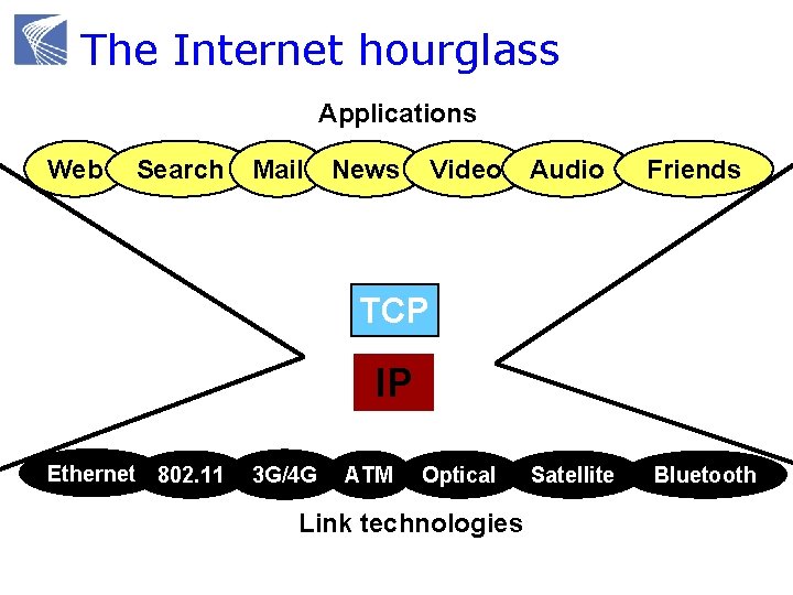
The Internet hourglass Applications Web Search Mail News Video Audio Friends TCP IP Ethernet 802. 11 3 G/4 G ATM Optical Link technologies Satellite Bluetooth

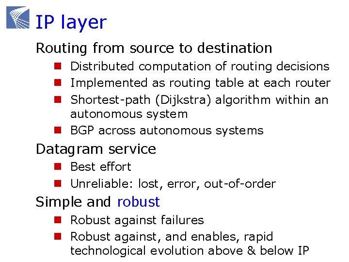
IP layer Routing from source to destination n Distributed computation of routing decisions n Implemented as routing table at each router n Shortest-path (Dijkstra) algorithm within an autonomous system n BGP across autonomous systems Datagram service n Best effort n Unreliable: lost, error, out-of-order Simple and robust n Robust against failures n Robust against, and enables, rapid technological evolution above & below IP

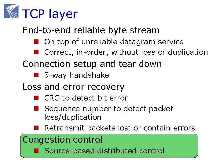
TCP layer End-to-end reliable byte stream n On top of unreliable datagram service n Correct, in-order, without loss or duplication Connection setup and tear down n 3 -way handshake Loss and error recovery n CRC to detect bit error n Sequence number to detect packet loss/duplication n Retransmit packets lost or contain errors Congestion control n Source-based distributed control

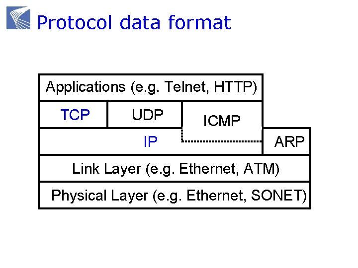
Protocol data format Applications (e. g. Telnet, HTTP) TCP UDP IP ICMP ARP Link Layer (e. g. Ethernet, ATM) Physical Layer (e. g. Ethernet, SONET)

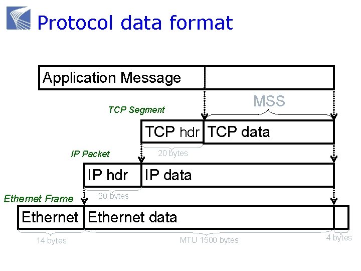
Protocol data format Application Message MSS TCP Segment TCP hdr TCP data IP Packet IP hdr Ethernet Frame 20 bytes IP data 20 bytes Ethernet data 14 bytes MTU 1500 bytes 4 bytes

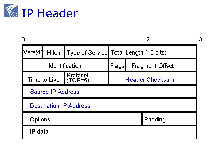
IP Header 0 1 2 Vers(4) H len Type of Service Total Length (16 bits) Identification Time to Live Protocol (TCP=6) Flags Fragment Offset Header Checksum Source IP Address Destination IP Address Options IP data Padding 3

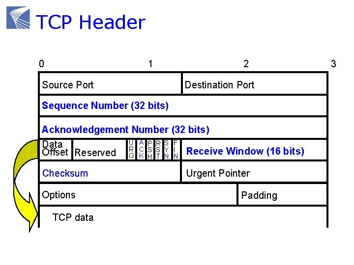
TCP Header 0 1 Source Port 2 Destination Port Sequence Number (32 bits) Acknowledgement Number (32 bits) U A P R S F Data C S S Y I Receive Window (16 bits) Offset Reserved R G K H T N N Checksum Options TCP data Urgent Pointer Padding 3

Congestion control protocols Why congestion control? Where is CC implemented? Window control mechanism CC protocols and basic structure Active queue management (AQM)

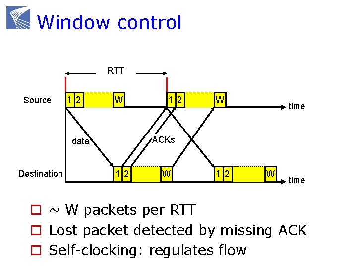
Window control RTT Source 1 2 W W time ACKs data Destination 1 2 W time o ~ W packets per RTT o Lost packet detected by missing ACK o Self-clocking: regulates flow

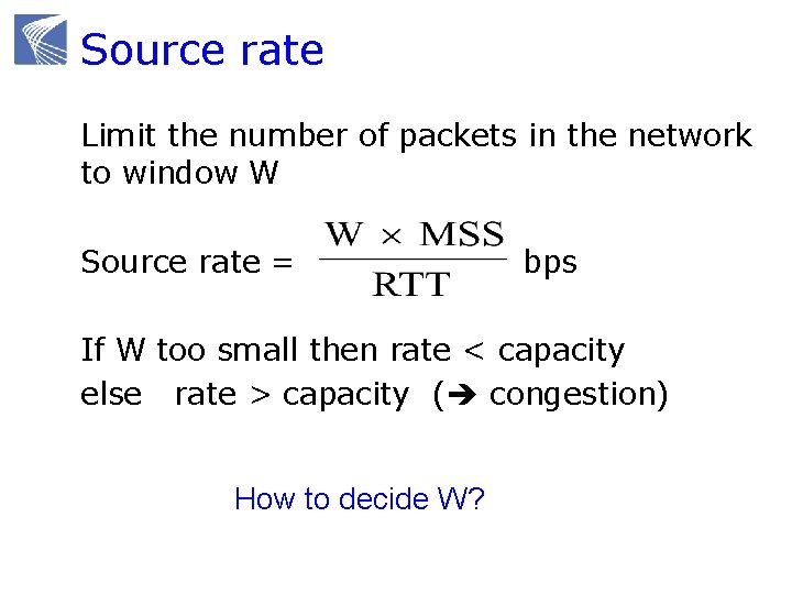
Source rate Limit the number of packets in the network to window W Source rate = bps If W too small then rate < capacity else rate > capacity ( congestion) How to decide W?

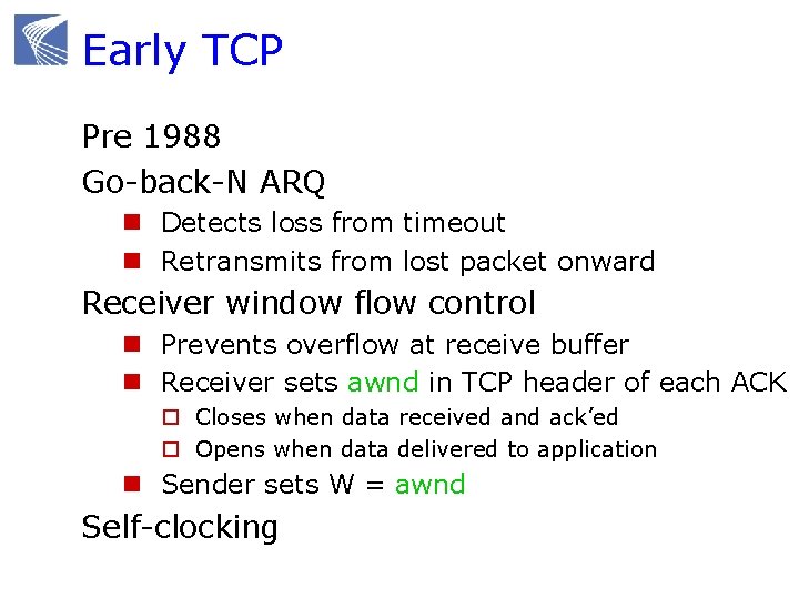
Early TCP Pre 1988 Go-back-N ARQ n Detects loss from timeout n Retransmits from lost packet onward Receiver window flow control n Prevents overflow at receive buffer n Receiver sets awnd in TCP header of each ACK o Closes when data received and ack’ed o Opens when data delivered to application n Sender sets W = awnd Self-clocking

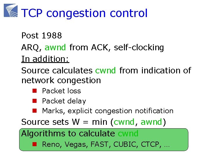
TCP congestion control Post 1988 ARQ, awnd from ACK, self-clocking In addition: Source calculates cwnd from indication of network congestion n Packet loss n Packet delay n Marks, explicit congestion notification Source sets W = min (cwnd, awnd) Algorithms to calculate cwnd n Reno, Vegas, FAST, CUBIC, CTCP, …

Congestion control protocols Why congestion control? Where is CC implemented? Window control mechanism CC protocols and basic structure Active queue management (AQM)

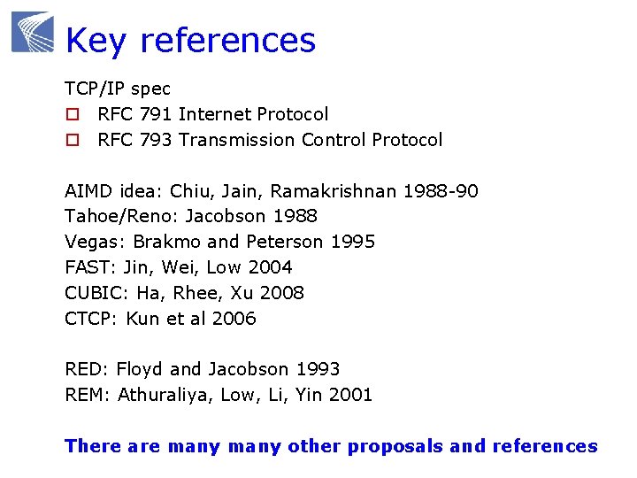
Key references TCP/IP spec o RFC 791 Internet Protocol o RFC 793 Transmission Control Protocol AIMD idea: Chiu, Jain, Ramakrishnan 1988 -90 Tahoe/Reno: Jacobson 1988 Vegas: Brakmo and Peterson 1995 FAST: Jin, Wei, Low 2004 CUBIC: Ha, Rhee, Xu 2008 CTCP: Kun et al 2006 RED: Floyd and Jacobson 1993 REM: Athuraliya, Low, Li, Yin 2001 There are many other proposals and references

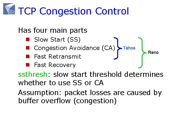
TCP Congestion Control Has four main parts n n Slow Start (SS) Congestion Avoidance (CA) Fast Retransmit Fast Recovery Tahoe Reno ssthresh: slow start threshold determines whether to use SS or CA Assumption: packet losses are caused by buffer overflow (congestion)

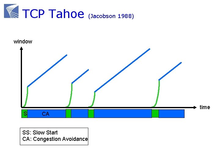
TCP Tahoe (Jacobson 1988) window time SS CA SS: Slow Start CA: Congestion Avoidance

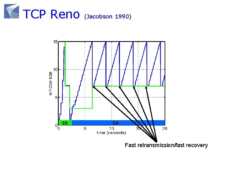
TCP Reno SS (Jacobson 1990) CA Fast retransmission/fast recovery

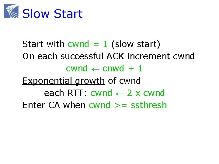
Slow Start with cwnd = 1 (slow start) On each successful ACK increment cwnd cnwd + 1 Exponential growth of cwnd each RTT: cwnd 2 x cwnd Enter CA when cwnd >= ssthresh

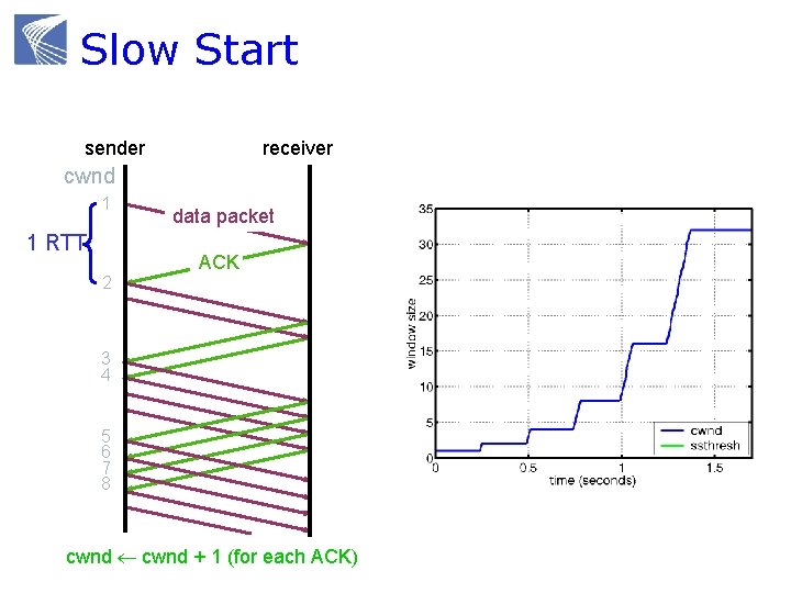
Slow Start sender receiver cwnd 1 1 RTT 2 data packet ACK 3 4 5 6 7 8 cwnd + 1 (for each ACK)

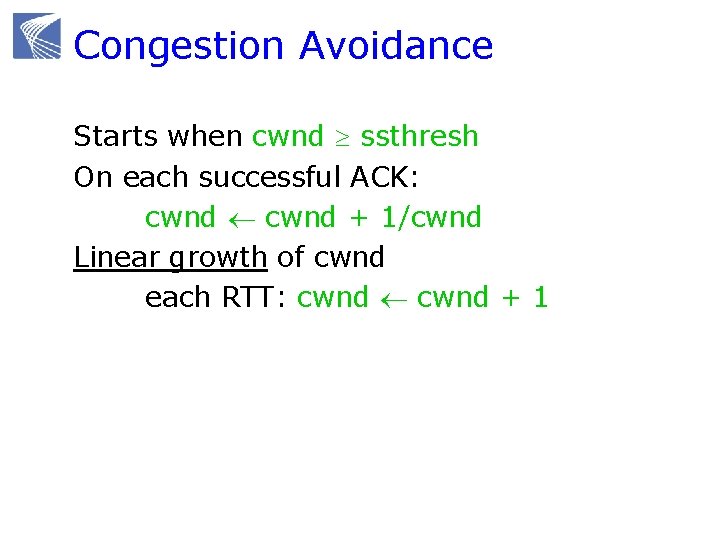
Congestion Avoidance Starts when cwnd ssthresh On each successful ACK: cwnd + 1/cwnd Linear growth of cwnd each RTT: cwnd + 1

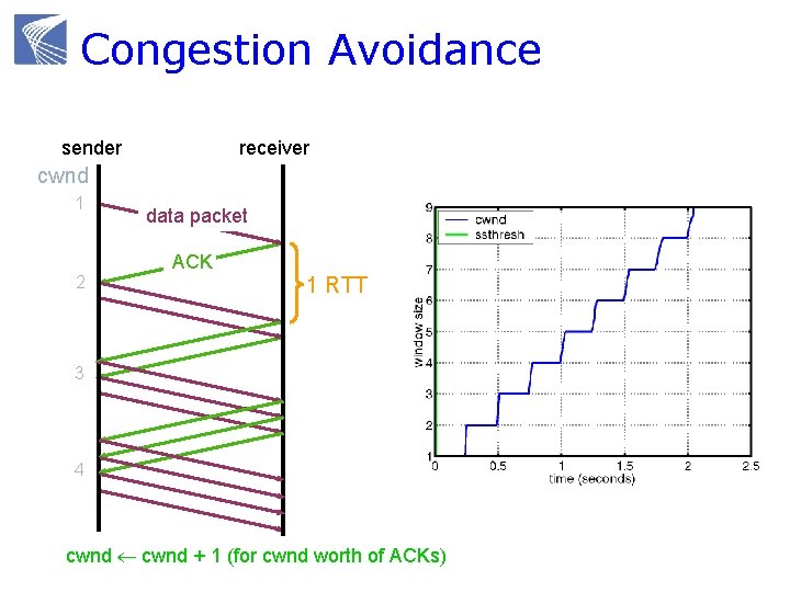
Congestion Avoidance sender receiver cwnd 1 2 data packet ACK 1 RTT 3 4 cwnd + 1 (for cwnd worth of ACKs)

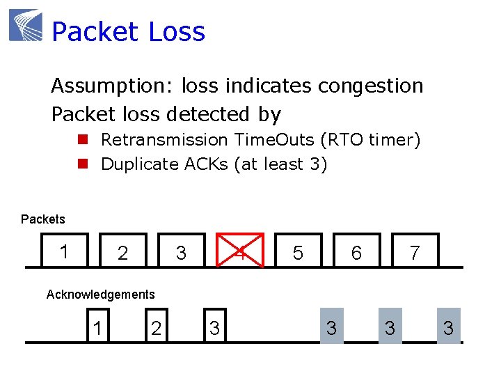
Packet Loss Assumption: loss indicates congestion Packet loss detected by n Retransmission Time. Outs (RTO timer) n Duplicate ACKs (at least 3) Packets 1 2 3 4 5 7 6 Acknowledgements 1 2 3 3

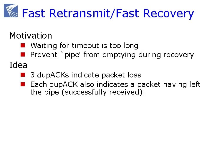
Fast Retransmit/Fast Recovery Motivation n Waiting for timeout is too long n Prevent `pipe’ from emptying during recovery Idea n 3 dup. ACKs indicate packet loss n Each dup. ACK also indicates a packet having left the pipe (successfully received)!

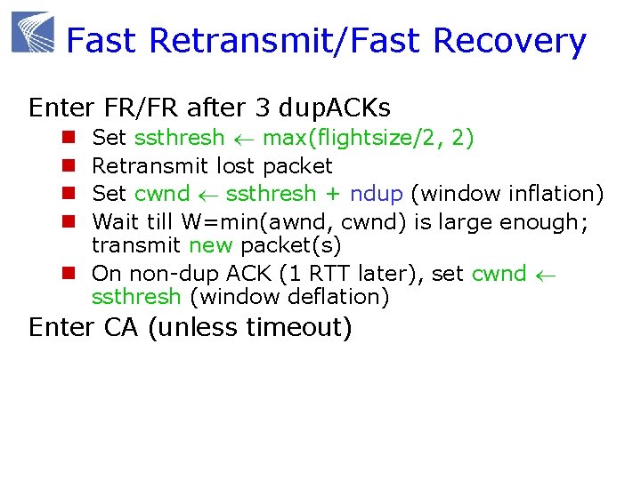
Fast Retransmit/Fast Recovery Enter FR/FR after 3 dup. ACKs Set ssthresh max(flightsize/2, 2) Retransmit lost packet Set cwnd ssthresh + ndup (window inflation) Wait till W=min(awnd, cwnd) is large enough; transmit new packet(s) n On non-dup ACK (1 RTT later), set cwnd ssthresh (window deflation) n n Enter CA (unless timeout)

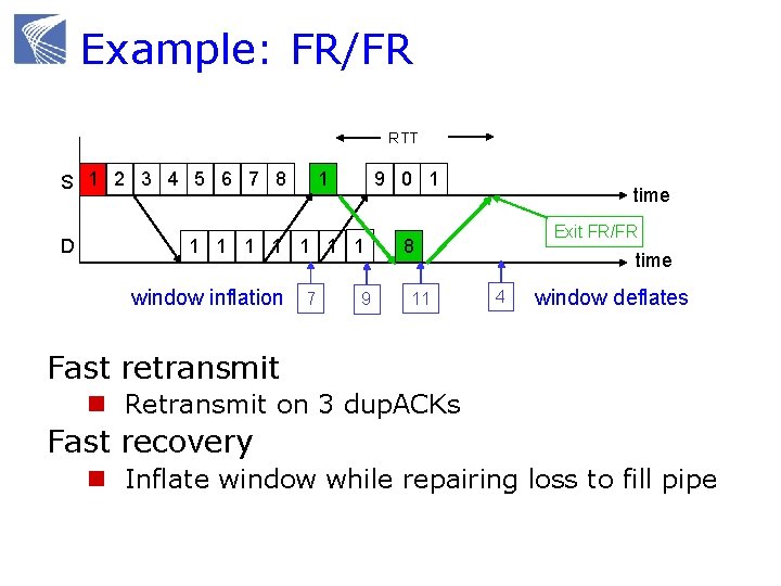
Example: FR/FR RTT S 1 2 3 4 5 6 7 8 D 1 9 0 1 1 1 1 window inflation 7 9 time Exit FR/FR 8 11 time 4 window deflates Fast retransmit n Retransmit on 3 dup. ACKs Fast recovery n Inflate window while repairing loss to fill pipe

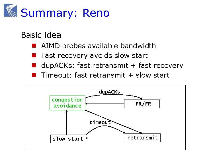
Summary: Reno Basic idea n n AIMD probes available bandwidth Fast recovery avoids slow start dup. ACKs: fast retransmit + fast recovery Timeout: fast retransmit + slow start dup. ACKs congestion avoidance FR/FR timeout slow start retransmit

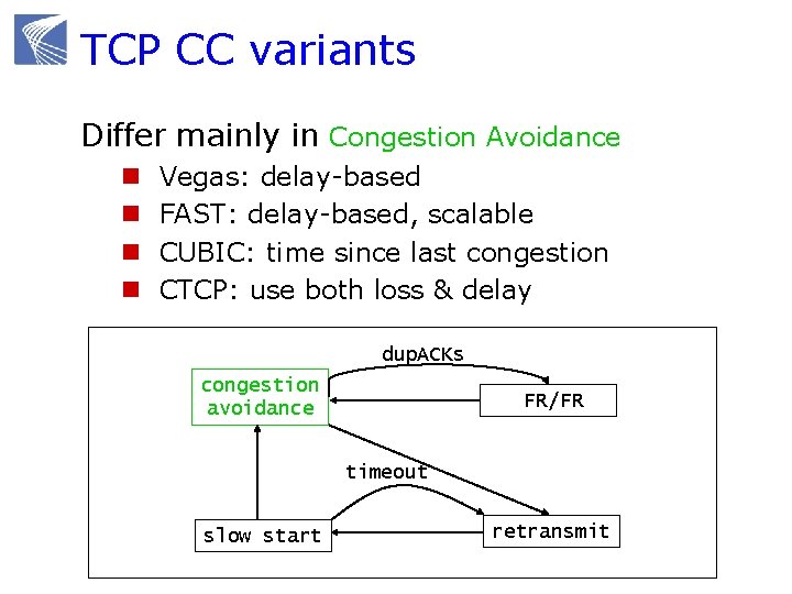
TCP CC variants Differ mainly in Congestion Avoidance n n Vegas: delay-based FAST: delay-based, scalable CUBIC: time since last congestion CTCP: use both loss & delay dup. ACKs congestion avoidance FR/FR timeout slow start retransmit

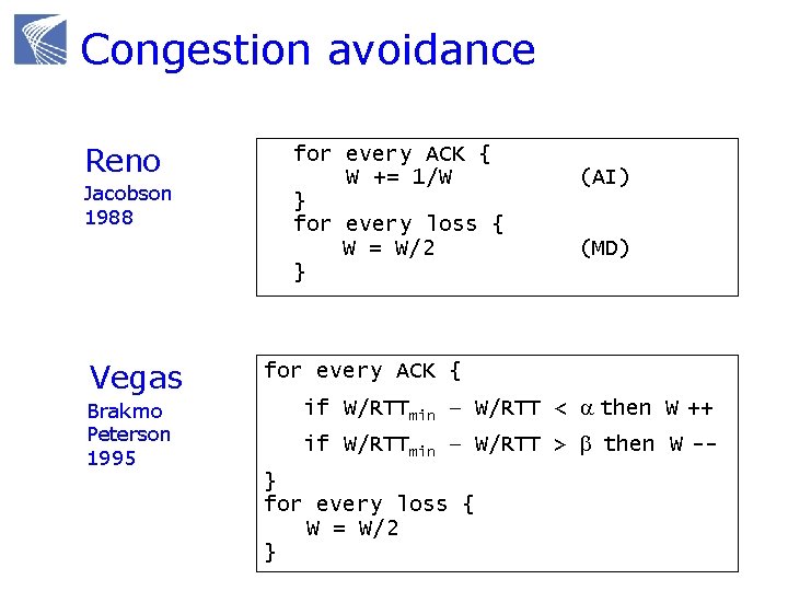
Congestion avoidance Reno Jacobson 1988 Vegas Brakmo Peterson 1995 for every ACK { W += 1/W } for every loss { W = W/2 } (AI) (MD) for every ACK { if W/RTTmin – W/RTT < a then W ++ if W/RTTmin – W/RTT > b then W -} for every loss { W = W/2 }

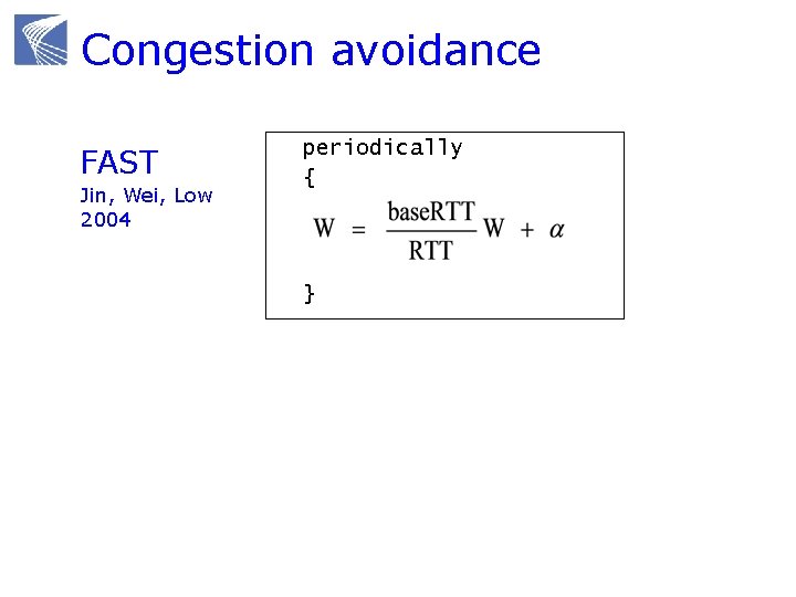
Congestion avoidance FAST Jin, Wei, Low 2004 periodically { }

Congestion control protocols Why congestion control? Where is CC implemented? Window control mechanism CC protocols and basic structure Active queue management (AQM)

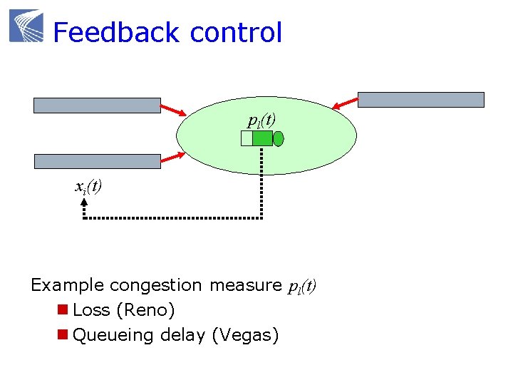
Feedback control pl(t) xi(t) Example congestion measure pl(t) n Loss (Reno) n Queueing delay (Vegas)

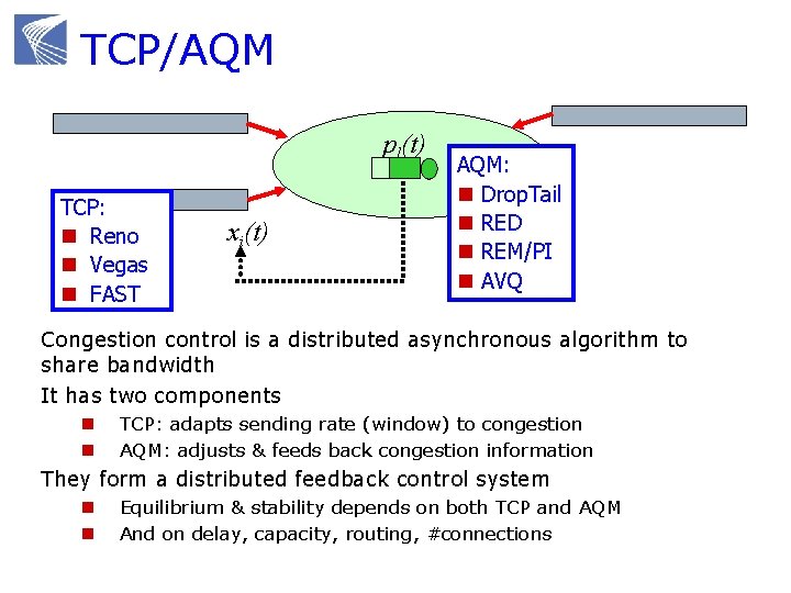
TCP/AQM pl(t) TCP: n Reno n Vegas n FAST xi(t) AQM: n Drop. Tail n RED n REM/PI n AVQ Congestion control is a distributed asynchronous algorithm to share bandwidth It has two components n n TCP: adapts sending rate (window) to congestion AQM: adjusts & feeds back congestion information They form a distributed feedback control system n n Equilibrium & stability depends on both TCP and AQM And on delay, capacity, routing, #connections

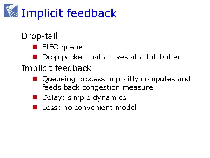
Implicit feedback Drop-tail n FIFO queue n Drop packet that arrives at a full buffer Implicit feedback n Queueing process implicitly computes and feeds back congestion measure n Delay: simple dynamics n Loss: no convenient model

Active queue management Explicit feedback n Provide congestion information by probabilistically marking packets n 2 ECN bit in IP header allocated for AQM Supported by all new routers but usually turned off in the field

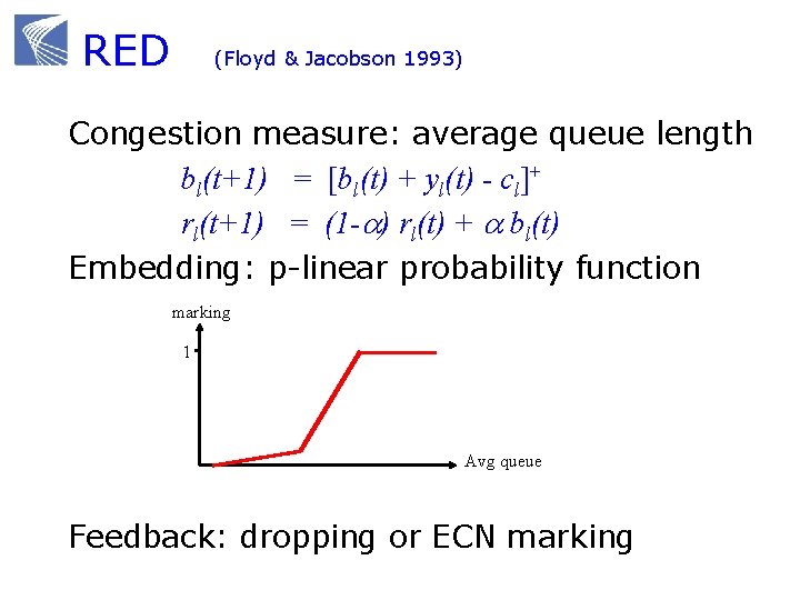
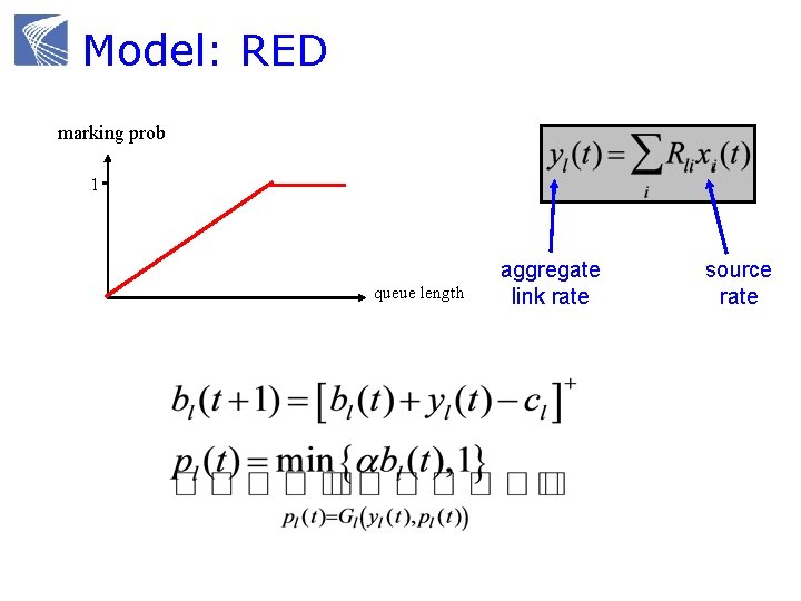
RED (Floyd & Jacobson 1993) Congestion measure: average queue length bl(t+1) = [bl(t) + yl(t) - cl]+ rl(t+1) = (1 -a) rl(t) + a bl(t) Embedding: p-linear probability function marking 1 Avg queue Feedback: dropping or ECN marking

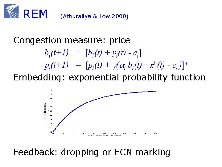
REM (Athuraliya & Low 2000) Congestion measure: price bl(t+1) = [bl(t) + yl(t) - cl]+ pl(t+1) = [pl(t) + g(al bl(t)+ xl (t) - cl )]+ Embedding: exponential probability function Feedback: dropping or ECN marking

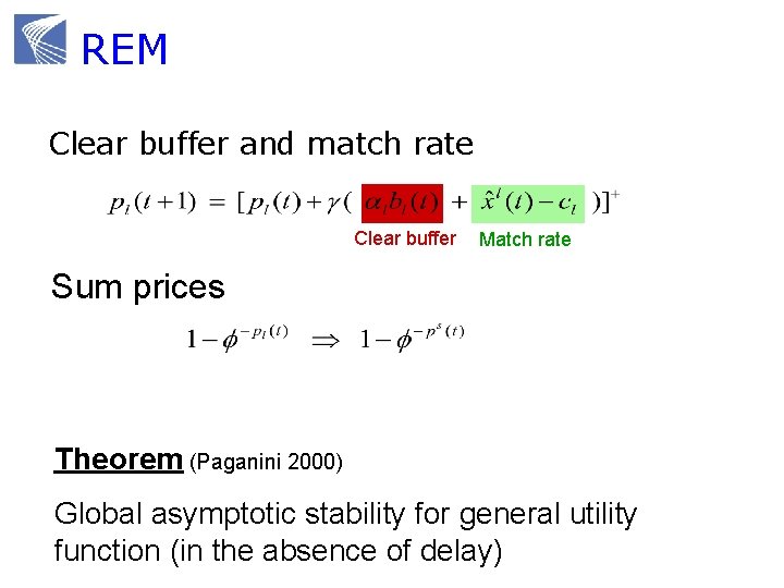
REM Clear buffer and match rate Clear buffer Match rate Sum prices Theorem (Paganini 2000) Global asymptotic stability for general utility function (in the absence of delay)

Summary: CC protocols End-to-end CC implemented in TCP n Basic window mechanism n TCP performs connection setup, error recovery, and congestion control, n CC dynamically computes cwnd that limits max #pkts enroute Distributed feedback control algorithm n TCP: adapts congestion window n AQM: adapts congestion measure

Agenda 9: 00 10: 00 Congestion control protocols break 10: 15 11: 15 Mathematical models break 11: 30 12: 30 Advanced topics lunch

MATHEMATICAL MODELS

Mathematical models Why mathematical models? Dynamical systems model of CC Convex optimization primer Reverse engr: equilibrium properties Forward engr: FAST TCP

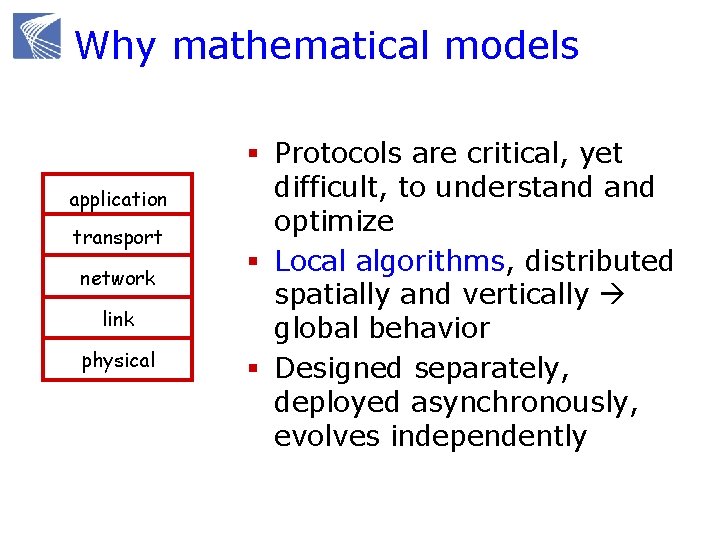
Why mathematical models application transport network link physical § Protocols are critical, yet difficult, to understand optimize § Local algorithms, distributed spatially and vertically global behavior § Designed separately, deployed asynchronously, evolves independently

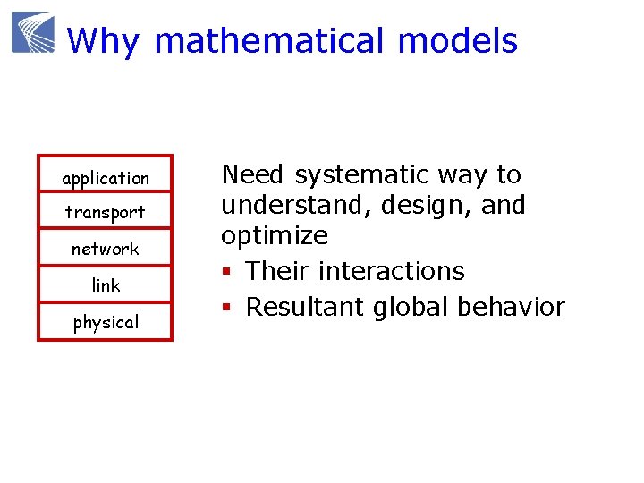
Why mathematical models application transport network link physical Need systematic way to understand, design, and optimize § Their interactions § Resultant global behavior

Why mathematical models Not to replace intuitions, expts, heuristics Provides structure and clarity n n n Refines intuition Guides design Suggests ideas Explores boundaries Understands structural properties Risk n “All models are wrong” n “… some are useful” n Validate with simulations & experiments

Structural properties Equilibrium properties n Throughput, delay, loss, fairness Dynamic properties n Stability n Robustness n Responsiveness Scalability properties n Information scaling (decentralization) n Computation scaling n Performance scaling

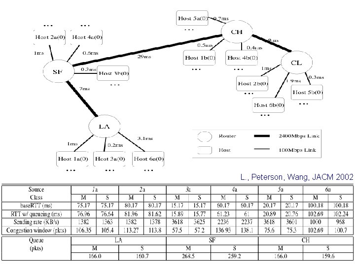
L. , Peterson, Wang, JACM 2002

Limitations of basic model Static and deterministic network n Fixed set of flows, link capacities, routing n Real networks are time-varying and random Homogeneous protocols n All flows use the same congestion measure Fluid approximation n Ignore packet level effects, e. g. burstiness n Inaccurate buffering process Difficulty in analysis of model basic stability model has been generalized n Global in presence of feedback delay to address these issues to various degrees n Robustness, responsiveness

Mathematical models Why mathematical models? Dynamical systems model of CC Convex optimization primer Reverse engr: equilibrium properties Forward engr: FAST TCP

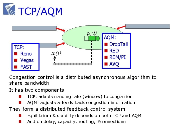
TCP/AQM pl(t) TCP: n Reno n Vegas n FAST xi(t) AQM: n Drop. Tail n RED n REM/PI n AVQ Congestion control is a distributed asynchronous algorithm to share bandwidth It has two components n n TCP: adapts sending rate (window) to congestion AQM: adjusts & feeds back congestion information They form a distributed feedback control system n n Equilibrium & stability depends on both TCP and AQM And on delay, capacity, routing, #connections

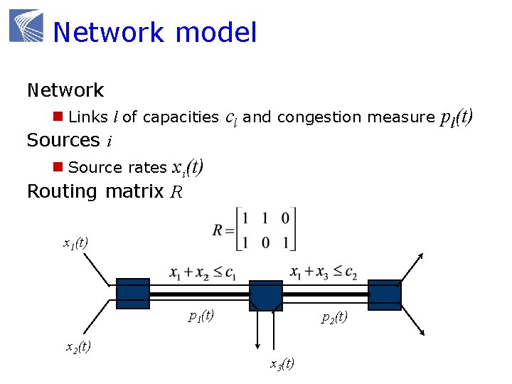
Network model Network n Links l of capacities cl and congestion measure pl(t) Sources i n Source rates xi(t) Routing matrix R x 1(t) p 1(t) x 2(t) p 2(t) x 3(t)

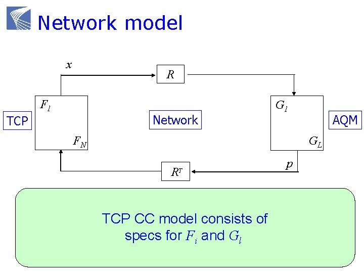
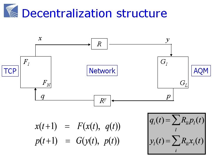
Network model x y R F 1 Network TCP G 1 FN q AQM GL R T p IP routing TCP CC model consists of specs for Fi and Gl Reno, Vegas Droptail, RED

Examples Derive (Fi, Gl) model for n Reno/RED n Vegas/Droptail n FAST/Droptail Focus on Congestion Avoidance

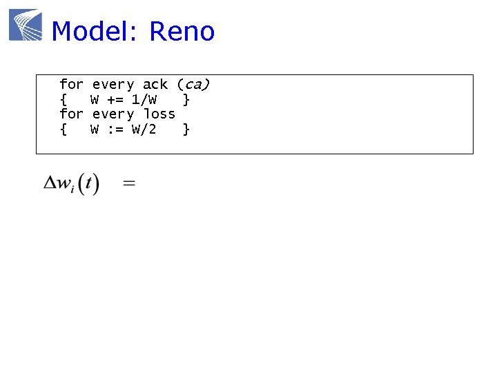
Model: Reno for { every ack (ca) W += 1/W } every loss W : = W/2 }

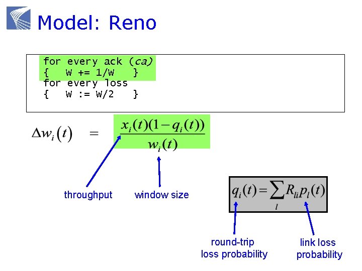
Model: Reno for { every ack (ca) W += 1/W } every loss W : = W/2 } throughput window size round-trip loss probability link loss probability

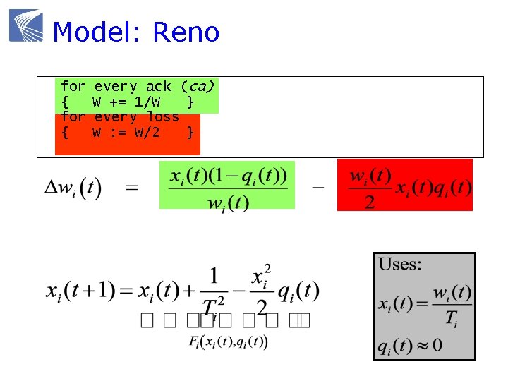
Model: Reno for { every ack (ca) W += 1/W } every loss W : = W/2 }

Model: RED marking prob 1 queue length aggregate link rate source rate

Model: Reno/RED

Decentralization structure x yy R F 1 Network TCP G 1 FN qq AQM GL R T p

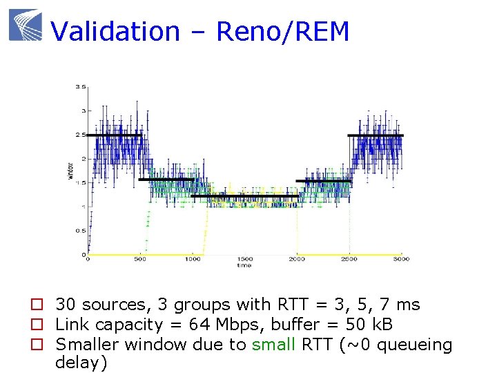
Validation – Reno/REM o 30 sources, 3 groups with RTT = 3, 5, 7 ms o Link capacity = 64 Mbps, buffer = 50 k. B o Smaller window due to small RTT (~0 queueing delay)

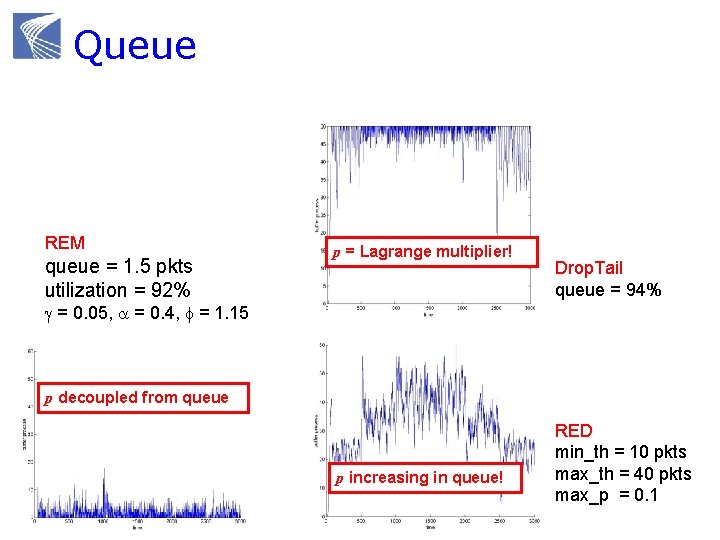
Queue REM queue = 1. 5 pkts utilization = 92% p = Lagrange multiplier! Drop. Tail queue = 94% g = 0. 05, a = 0. 4, f = 1. 15 p decoupled from queue p increasing in queue! RED min_th = 10 pkts max_th = 40 pkts max_p = 0. 1

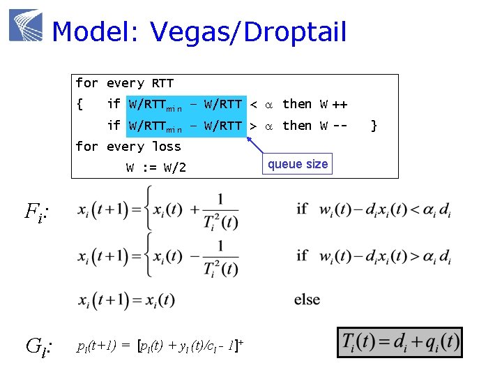
Model: Vegas/Droptail for every RTT { if W/RTTmin – W/RTT < a then W ++ if W/RTTmin – W/RTT > a then W -- for every loss W : = W/2 F i: Gl : pl(t+1) = [pl(t) + yl (t)/cl - 1]+ queue size }

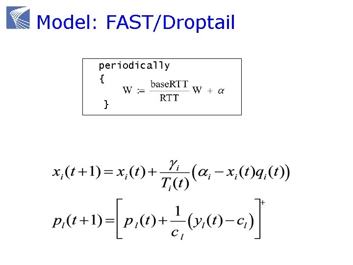
Model: FAST/Droptail periodically { }

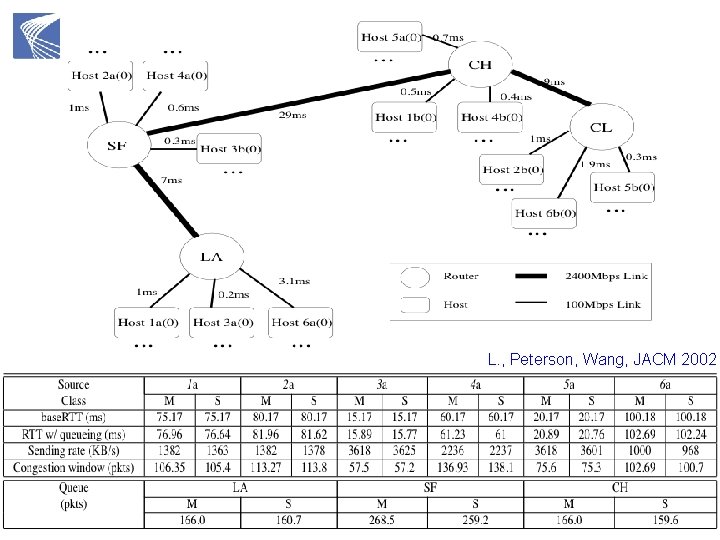
L. , Peterson, Wang, JACM 2002

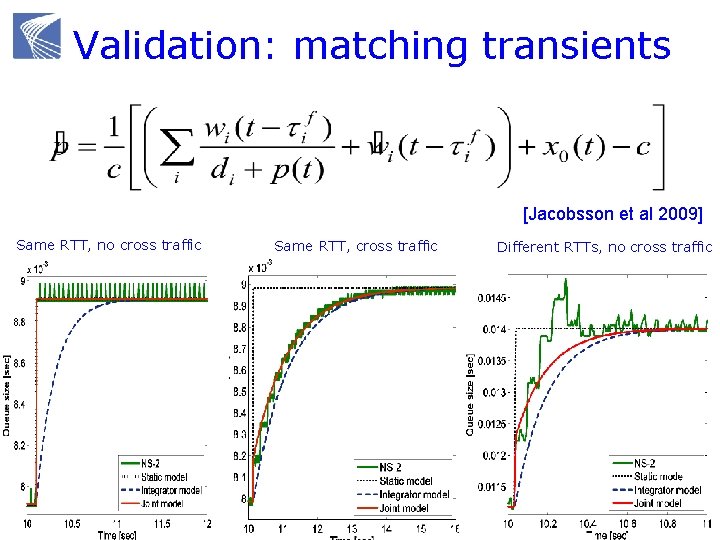
Validation: matching transients [Jacobsson et al 2009] Same RTT, no cross traffic Same RTT, cross traffic Different RTTs, no cross traffic

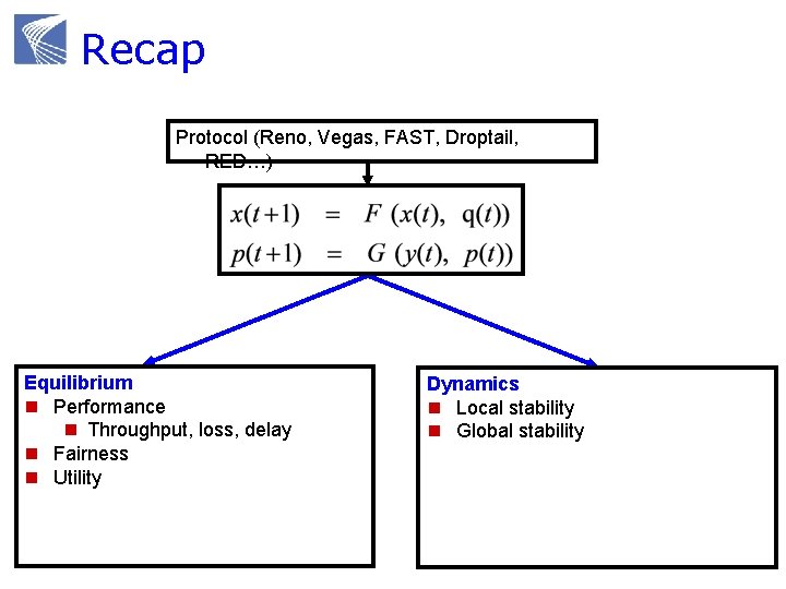
Recap Protocol (Reno, Vegas, FAST, Droptail, RED…) Equilibrium n Performance n Throughput, loss, delay n Fairness n Utility Dynamics n Local stability n Global stability

Mathematical models Why mathematical models? Dynamical systems model of CC Convex optimization primer Reverse engr: equilibrium properties Forward engr: FAST TCP

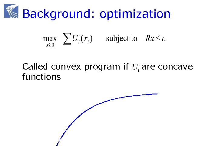
Background: optimization Called convex program if Ui are concave functions

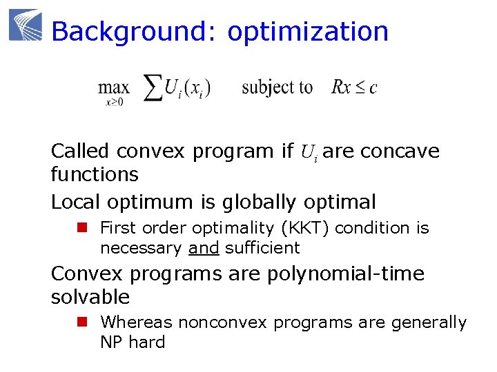
Background: optimization Called convex program if Ui are concave functions Local optimum is globally optimal n First order optimality (KKT) condition is necessary and sufficient Convex programs are polynomial-time solvable n Whereas nonconvex programs are generally NP hard

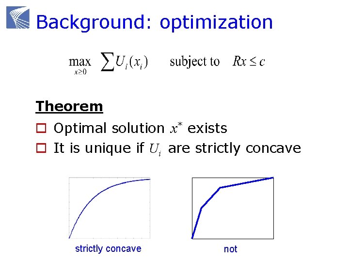
Background: optimization Theorem o Optimal solution x* exists o It is unique if Ui are strictly concave not

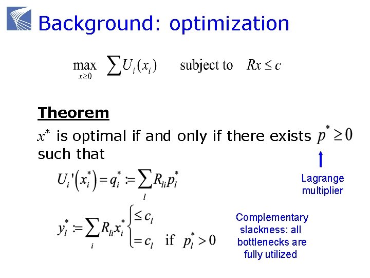
Background: optimization Theorem x* is optimal if and only if there exists such that Lagrange multiplier Complementary slackness: all bottlenecks are fully utilized

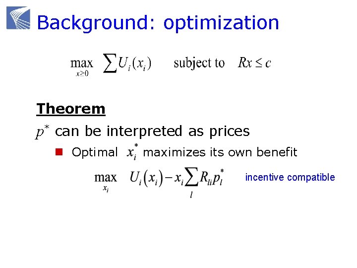
Background: optimization Theorem p* can be interpreted as prices n Optimal maximizes its own benefit incentive compatible

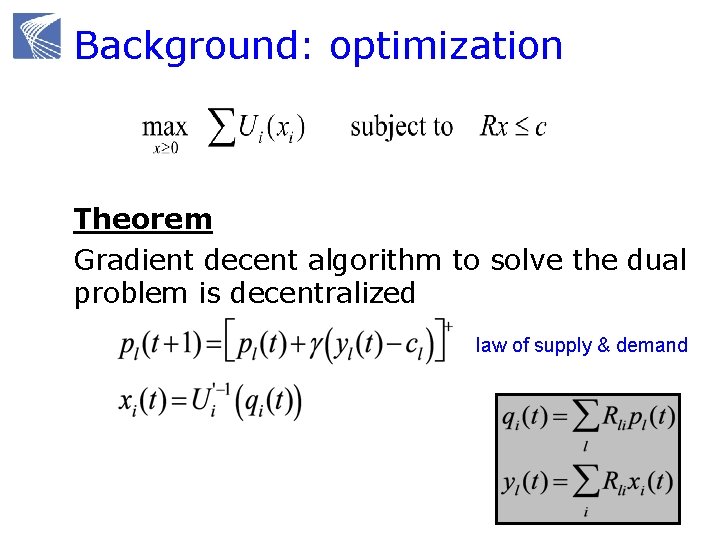
Background: optimization Theorem Gradient decent algorithm to solve the dual problem is decentralized law of supply & demand

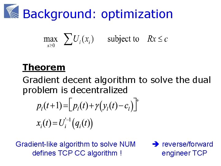
Background: optimization Theorem Gradient decent algorithm to solve the dual problem is decentralized Gradient-like algorithm to solve NUM defines TCP CC algorithm ! reverse/forward engineer TCP

Mathematical models Why mathematical models? Dynamical systems model of CC Convex optimization primer Reverse engr: equilibrium properties Forward engr: FAST TCP

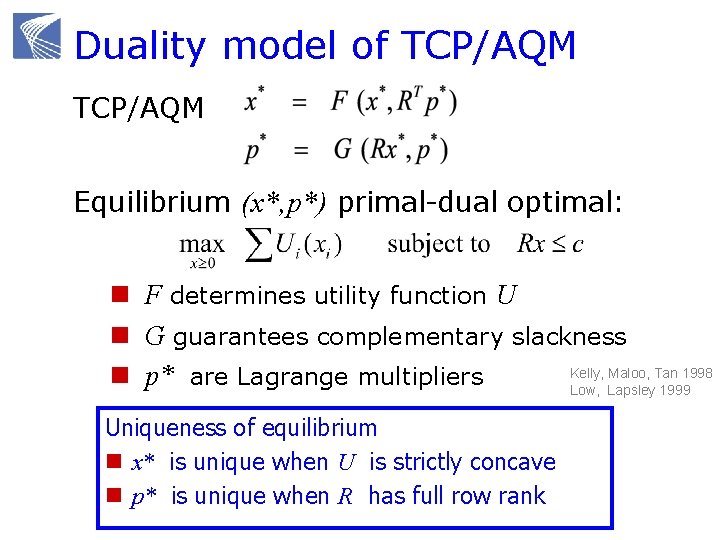
Duality model of TCP/AQM Equilibrium (x*, p*) primal-dual optimal: n F determines utility function U n G guarantees complementary slackness Kelly, Maloo, Tan 1998 n p* are Lagrange multipliers Low, Lapsley 1999 Uniqueness of equilibrium n x* is unique when U is strictly concave n p* is unique when R has full row rank

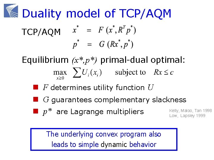
Duality model of TCP/AQM Equilibrium (x*, p*) primal-dual optimal: n F determines utility function U n G guarantees complementary slackness Kelly, Maloo, Tan 1998 n p* are Lagrange multipliers Low, Lapsley 1999 The underlying convex program also leads to simple dynamic behavior

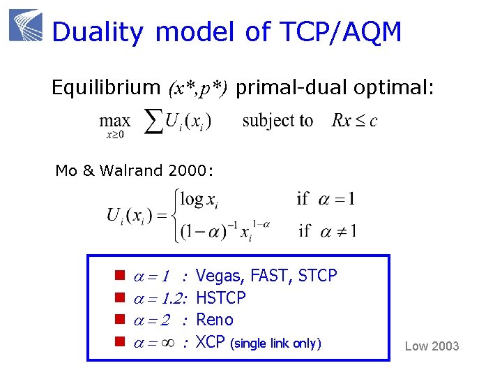
Duality model of TCP/AQM Equilibrium (x*, p*) primal-dual optimal: Mo & Walrand 2000: n n a=1 : a = 1. 2: a=2 : a= : Vegas, FAST, STCP HSTCP Reno XCP (single link only) Low 2003

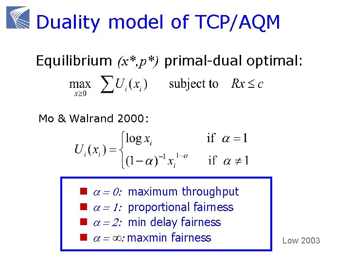
Duality model of TCP/AQM Equilibrium (x*, p*) primal-dual optimal: Mo & Walrand 2000: n n a = 0: maximum throughput a = 1: proportional fairness a = 2: min delay fairness a = : maxmin fairness Low 2003

Some implications Equilibrium n Always exists, unique if R is full rank n Bandwidth allocation independent of AQM or arrival n Can predict macroscopic behavior of large scale networks Counter-intuitive throughput behavior n Fair allocation is not always inefficient n Increasing link capacities do not always raise aggregate throughput [Tang, Wang, Low, To. N 2006] Forward engineering: FAST TCP n Design, analysis, experiments [Wei, Jin, Low, Hegde, To. N 2006]

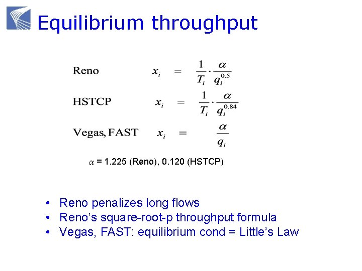
Equilibrium throughput a = 1. 225 (Reno), 0. 120 (HSTCP) • Reno penalizes long flows • Reno’s square-root-p throughput formula • Vegas, FAST: equilibrium cond = Little’s Law

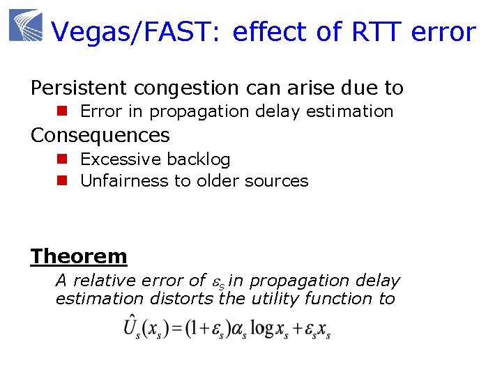
Vegas/FAST: effect of RTT error Persistent congestion can arise due to n Error in propagation delay estimation Consequences n Excessive backlog n Unfairness to older sources Theorem A relative error of es in propagation delay estimation distorts the utility function to

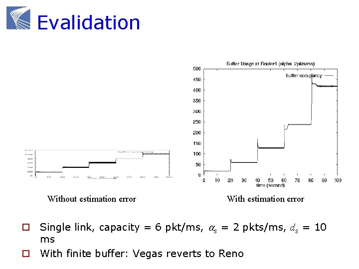
Evalidation Without estimation error With estimation error o Single link, capacity = 6 pkt/ms, as = 2 pkts/ms, ds = 10 ms o With finite buffer: Vegas reverts to Reno

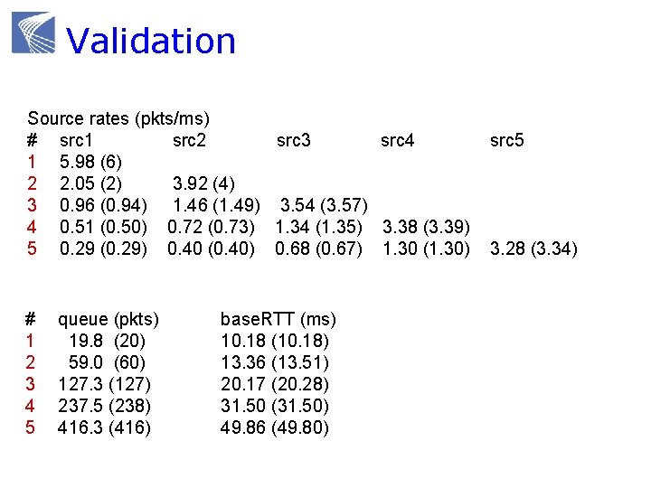
Validation Source rates (pkts/ms) # src 1 src 2 src 3 src 4 1 5. 98 (6) 2 2. 05 (2) 3. 92 (4) 3 0. 96 (0. 94) 1. 46 (1. 49) 3. 54 (3. 57) 4 0. 51 (0. 50) 0. 72 (0. 73) 1. 34 (1. 35) 3. 38 (3. 39) 5 0. 29 (0. 29) 0. 40 (0. 40) 0. 68 (0. 67) 1. 30 (1. 30) # 1 2 3 4 5 queue (pkts) 19. 8 (20) 59. 0 (60) 127. 3 (127) 237. 5 (238) 416. 3 (416) base. RTT (ms) 10. 18 (10. 18) 13. 36 (13. 51) 20. 17 (20. 28) 31. 50 (31. 50) 49. 86 (49. 80) src 5 3. 28 (3. 34)

Mathematical models Why mathematical models? Dynamical systems model of CC Convex optimization primer Reverse engr: equilibrium properties Forward engr: FAST TCP

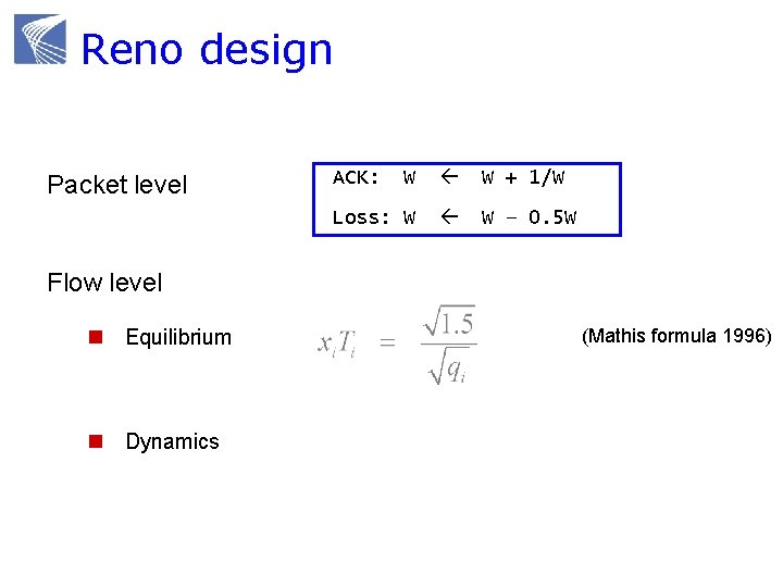
Reno design Reno TCP Packet level W W + 1/W Loss: W W – 0. 5 W ACK: Flow level n Equilibrium n Dynamics pkts (Mathis formula 1996)

Reno design Packet level n Designed and implemented first Flow level n Understood afterwards Flow level dynamics determines n Equilibrium: performance, fairness n Stability Design flow level equilibrium & stability Implement flow level goals at packet level

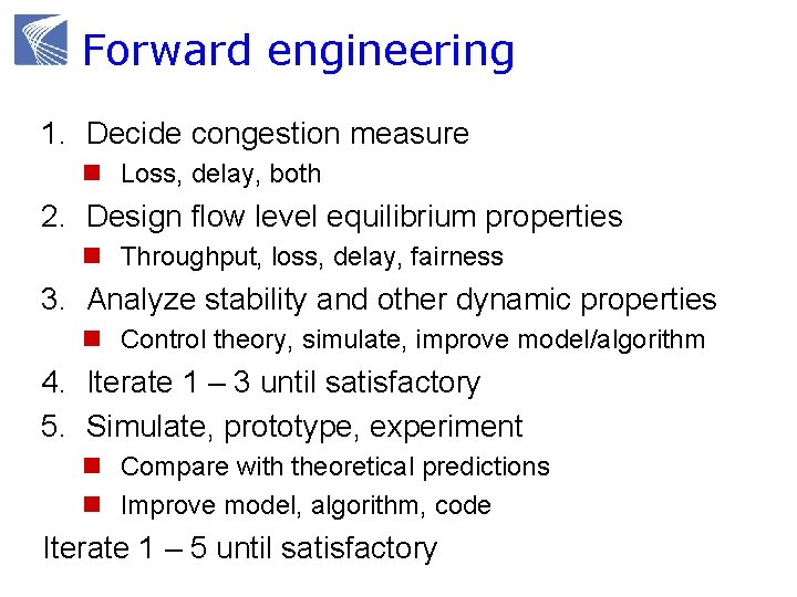
Forward engineering 1. Decide congestion measure n Loss, delay, both 2. Design flow level equilibrium properties n Throughput, loss, delay, fairness 3. Analyze stability and other dynamic properties n Control theory, simulate, improve model/algorithm 4. Iterate 1 – 3 until satisfactory 5. Simulate, prototype, experiment n Compare with theoretical predictions n Improve model, algorithm, code Iterate 1 – 5 until satisfactory

Forward engineering Tight integration of theory, design, experiment Performance analysis done at design time n Not after Theory does not replace intuitions and heuristics n Refines, validates/invalidates them Theory provides structure and clarity n Guides design n Suggests ideas and experiments n Explores boundaries that are hard to expt

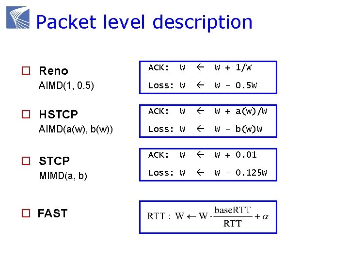
Packet level description o Reno AIMD(1, 0. 5) o HSTCP AIMD(a(w), b(w)) o STCP MIMD(a, b) o FAST W W + 1/W Loss: W W – 0. 5 W ACK: W W + a(w)/W Loss: W W – b(w)W ACK: W W + 0. 01 Loss: W W – 0. 125 W ACK:

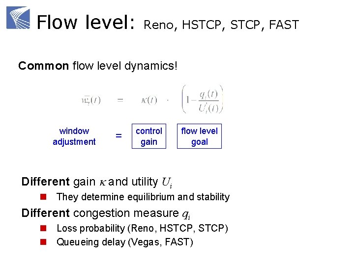
Flow level: Reno, HSTCP, FAST Common flow level dynamics! window adjustment = control gain flow level goal Different gain k and utility Ui n They determine equilibrium and stability Different congestion measure qi n Loss probability (Reno, HSTCP, STCP) n Queueing delay (Vegas, FAST)

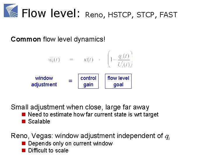
Flow level: Reno, HSTCP, FAST Common flow level dynamics! window adjustment = control gain flow level goal Small adjustment when close, large far away n Need to estimate how far current state is wrt target n Scalable Reno, Vegas: window adjustment independent of qi n Depends only on current window n Difficult to scale

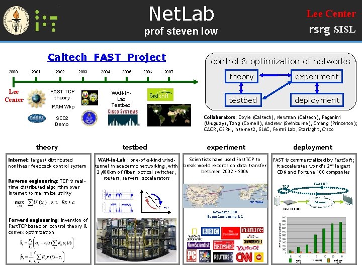
Net. Lab Lee Center rsrg SISL prof steven low Caltech FAST Project 2000 Lee Center 2001 2002 2003 FAST TCP theory IPAM Wkp 2004 2005 2006 2007 WAN-in. Lab Testbed Internet: largest distributed nonlinear feedback control system Reverse engineering: TCP is realtime distributed algorithm over Internet to maximize utility theory experiment testbed deployment Collaborators: Doyle (Caltech), Newman (Caltech), Paganini (Uruguay), Tang (Cornell), Andrew (Swinburne), Chiang (Princeton); CACR, CERN, Internet 2, SLAC, Fermi Lab, Star. Light, Cisco SC 02 Demo theory control & optimization of networks testbed WAN-in-Lab : one-of-a-kind windtunnel in academic networking, with 2, 400 km of fiber, optical switches, routers, servers, accelerators experiment deployment Scientists have used Fast. TCP to break world records on data transfer between 2002 – 2006 FAST is commercialized by Fast. Soft; it accelerates world’s 2 nd largest CDN and Fortune 100 companies eq 2 eq 3 SC 2004 eq 1 Forward engineering: Invention of Fast. TCP based on control theory & convex optimization Fast. TCP Internet 2 LSR Super. Computing BC Internet FAST in a box with FAST without FAST

Some benefits Transparent interaction among components n TCP, AQM n Clear understanding of structural properties Understanding effect of parameters n Change protocol parameters, topology, routing, link capacity, set of flows n Re-solve NUM n Systematic way to tune parameters

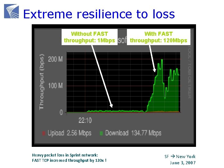
Extreme resilience to loss Without FAST throughput: 1 Mbps Heavy packet loss in Sprint network: FAST TCP increased throughput by 120 x ! With FAST throughput: 120 Mbps SF New York June 3, 2007

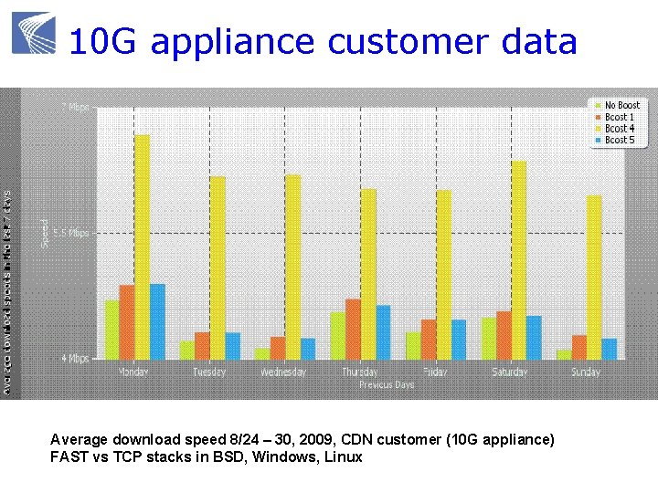
10 G appliance customer data Average download speed 8/24 – 30, 2009, CDN customer (10 G appliance) FAST vs TCP stacks in BSD, Windows, Linux

Summary: math models Integration of theory, design, experiment can be very powerful n Each needs the other n Combination much more than sum Theory-guided design approach n Tremendous progress in the last decade; not as impossible as most feared n Very difficult; but worth the effort n Most critical: mindset How to push theory-guided design approach further ?

Agenda 9: 00 10: 00 Congestion control protocols break 10: 15 11: 15 Mathematical models break 11: 30 12: 30 Advanced topics lunch

ADVANCED TOPICS

Advanced topics Heterogeneous protocols Layering as optimization decomposition

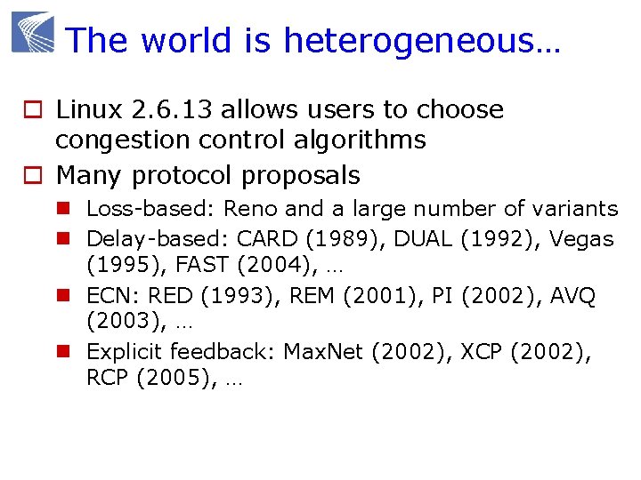
The world is heterogeneous… o Linux 2. 6. 13 allows users to choose congestion control algorithms o Many protocol proposals n Loss-based: Reno and a large number of variants n Delay-based: CARD (1989), DUAL (1992), Vegas (1995), FAST (2004), … n ECN: RED (1993), REM (2001), PI (2002), AVQ (2003), … n Explicit feedback: Max. Net (2002), XCP (2002), RCP (2005), …

Some implications homogeneous heterogeneous equilibrium unique ? bandwidth allocation on AQM independent ? bandwidth allocation on arrival independent ?

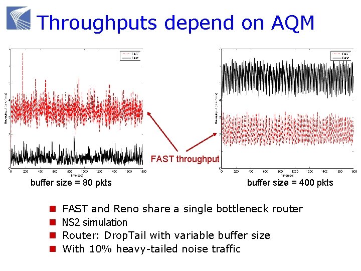
Throughputs depend on AQM FAST throughput buffer size = 80 pkts n n buffer size = 400 pkts FAST and Reno share a single bottleneck router NS 2 simulation Router: Drop. Tail with variable buffer size With 10% heavy-tailed noise traffic

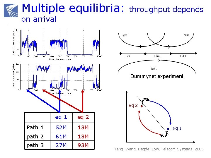
Multiple equilibria: throughput depends on arrival Dummynet experiment eq 2 eq 1 eq 2 Path 1 52 M 13 M path 2 61 M 13 M path 3 27 M 93 M eq 1 Tang, Wang, Hegde, Low, Telecom Systems, 2005

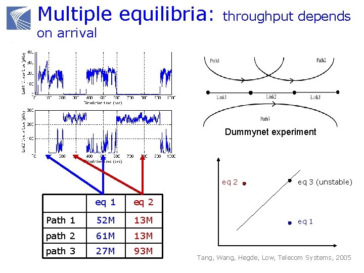
Multiple equilibria: throughput depends on arrival Dummynet experiment eq 2 eq 1 eq 2 Path 1 52 M 13 M path 2 61 M 13 M path 3 27 M 93 M eq 3 (unstable) eq 1 Tang, Wang, Hegde, Low, Telecom Systems, 2005

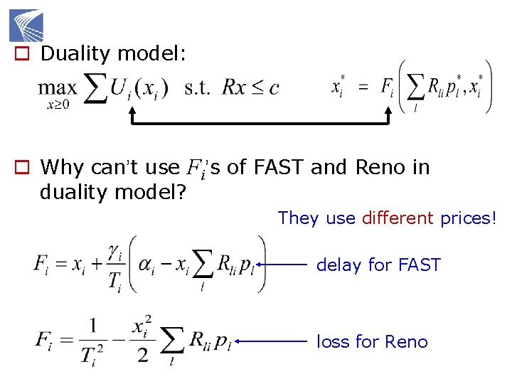
o Duality model: o Why can’t use Fi’s of FAST and Reno in duality model? They use different prices! delay for FAST loss for Reno

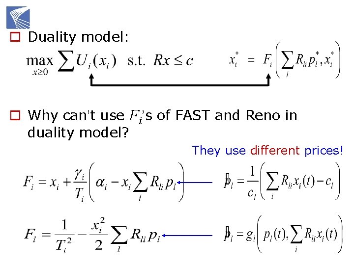
o Duality model: o Why can’t use Fi’s of FAST and Reno in duality model? They use different prices!

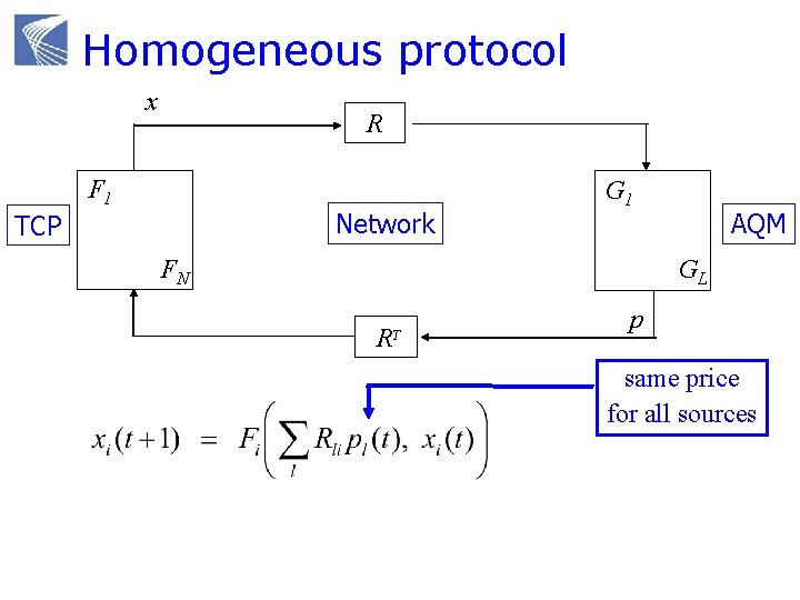
Homogeneous protocol x y R F 1 Network TCP G 1 FN q AQM GL R T p same price for all sources

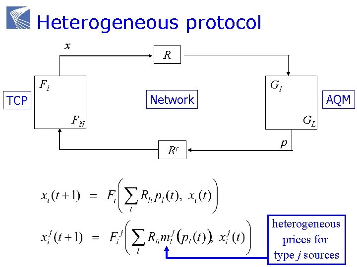
Heterogeneous protocol x y R F 1 Network TCP G 1 FN q AQM GL R T p heterogeneous prices for type j sources

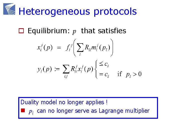
Heterogeneous protocols o Equilibrium: p that satisfies Duality model no longer applies ! n pl can no longer serve as Lagrange multiplier

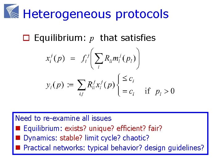
Heterogeneous protocols o Equilibrium: p that satisfies Need to re-examine all issues n Equilibrium: exists? unique? efficient? fair? n Dynamics: stable? limit cycle? chaotic? n Practical networks: typical behavior? design guidelines?

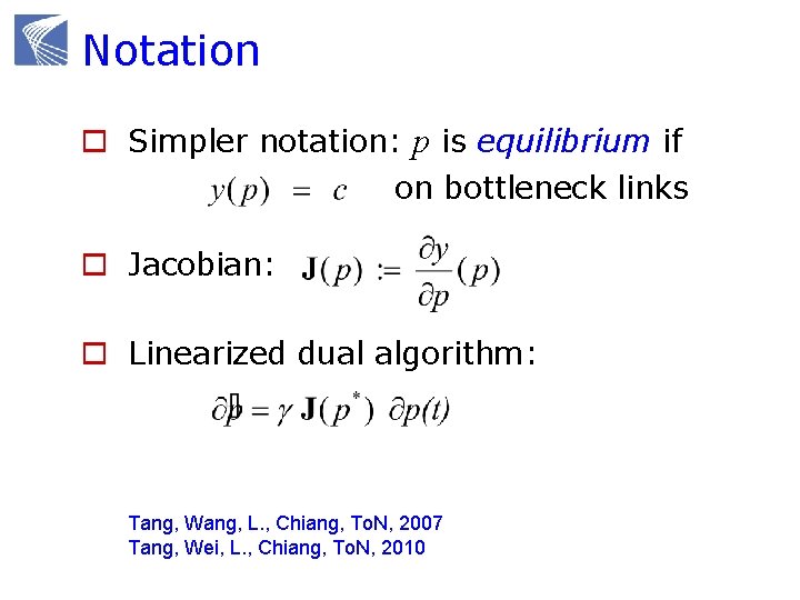
Notation o Simpler notation: p is equilibrium if on bottleneck links o Jacobian: o Linearized dual algorithm: Tang, Wang, L. , Chiang, To. N, 2007 Tang, Wei, L. , Chiang, To. N, 2010

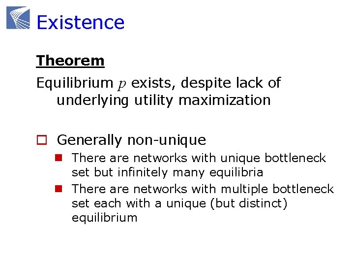
Existence Theorem Equilibrium p exists, despite lack of underlying utility maximization o Generally non-unique n There are networks with unique bottleneck set but infinitely many equilibria n There are networks with multiple bottleneck set each with a unique (but distinct) equilibrium

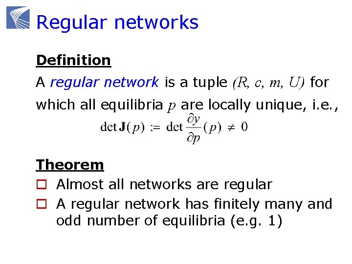
Regular networks Definition A regular network is a tuple (R, c, m, U) for which all equilibria p are locally unique, i. e. , Theorem o Almost all networks are regular o A regular network has finitely many and odd number of equilibria (e. g. 1)

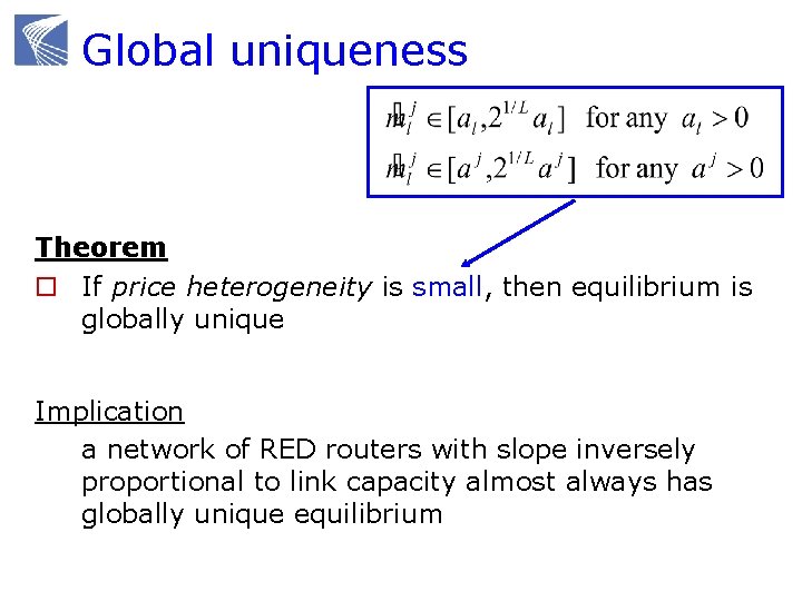
Global uniqueness Theorem o If price heterogeneity is small, then equilibrium is globally unique Implication a network of RED routers with slope inversely proportional to link capacity almost always has globally unique equilibrium

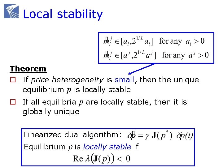
Local stability Theorem o If price heterogeneity is small, then the unique equilibrium p is locally stable o If all equilibria p are locally stable, then it is globally unique Linearized dual algorithm: Equilibrium p is locally stable if

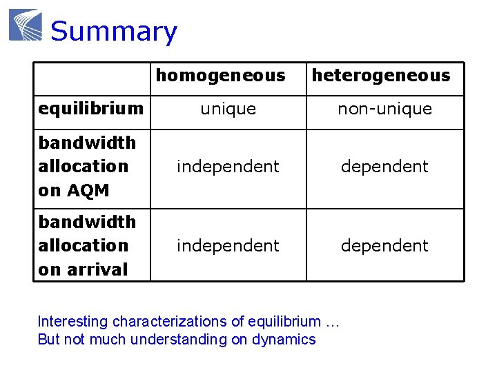
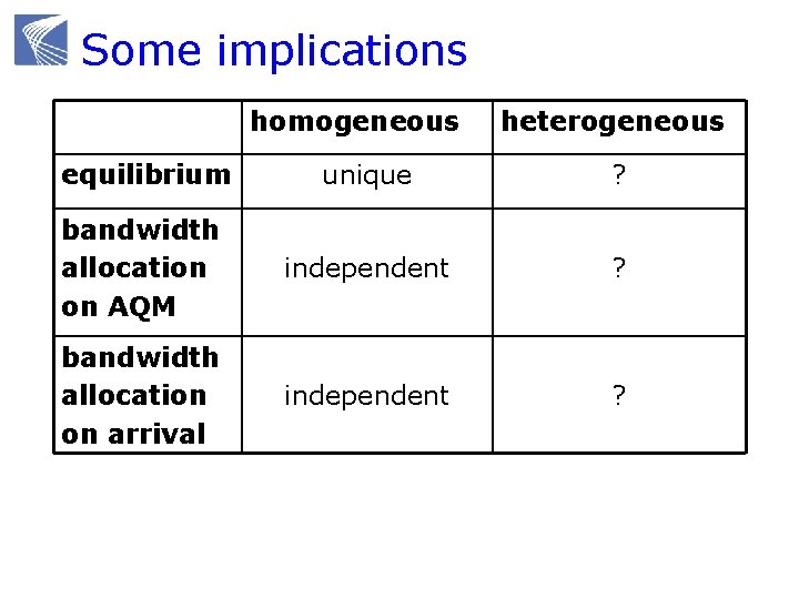
Summary homogeneous heterogeneous equilibrium unique non-unique bandwidth allocation on AQM independent bandwidth allocation on arrival independent Interesting characterizations of equilibrium … But not much understanding on dynamics

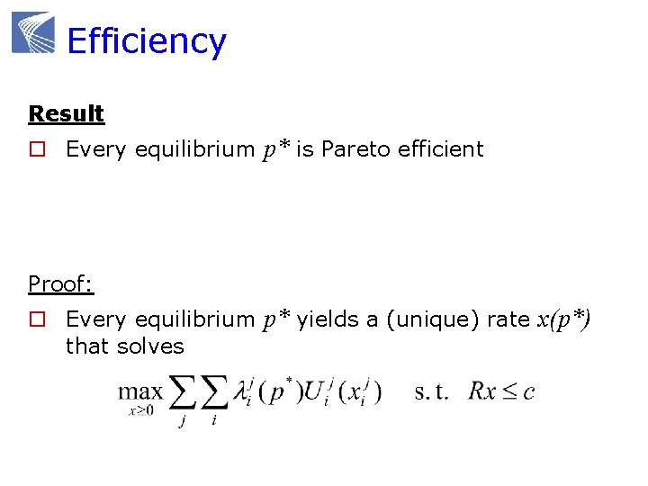
Efficiency Result o Every equilibrium p* is Pareto efficient Proof: o Every equilibrium p* yields a (unique) rate x(p*) that solves

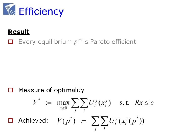
Efficiency Result o Every equilibrium p* is Pareto efficient o Measure of optimality o Achieved:

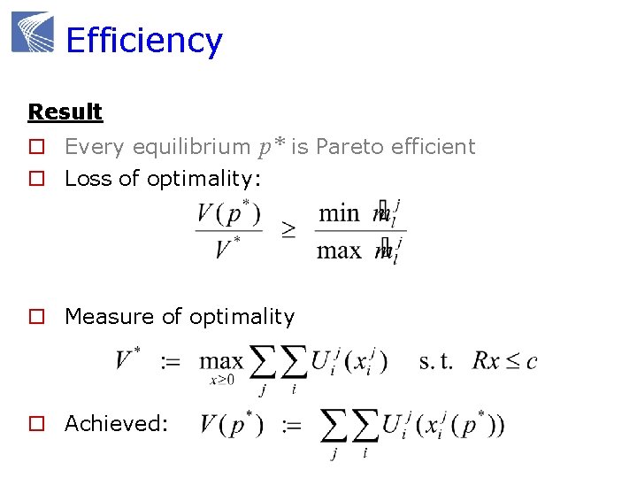
Efficiency Result o Every equilibrium p* is Pareto efficient o Loss of optimality: o Measure of optimality o Achieved:

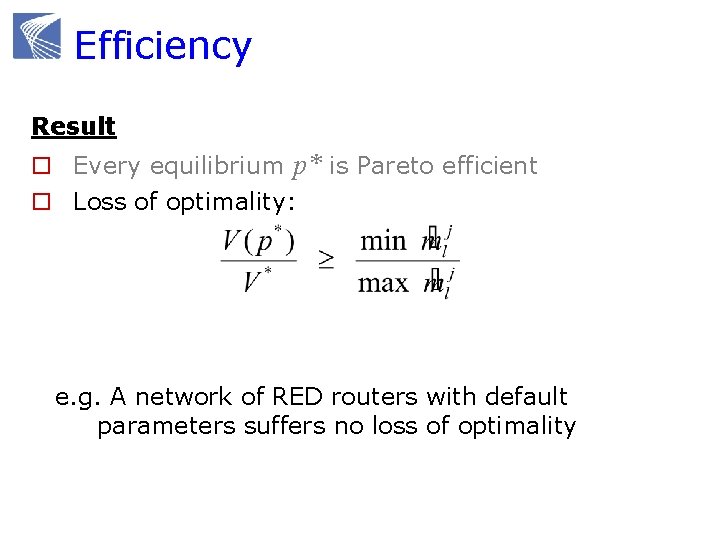
Efficiency Result o Every equilibrium p* is Pareto efficient o Loss of optimality: e. g. A network of RED routers with default parameters suffers no loss of optimality

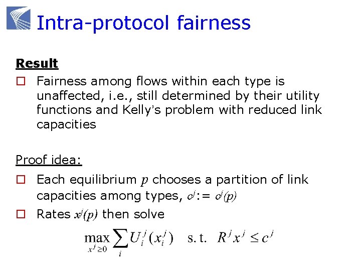
Intra-protocol fairness Result o Fairness among flows within each type is unaffected, i. e. , still determined by their utility functions and Kelly’s problem with reduced link capacities Proof idea: o Each equilibrium p chooses a partition of link capacities among types, cj: = cj(p) o Rates xj(p) then solve

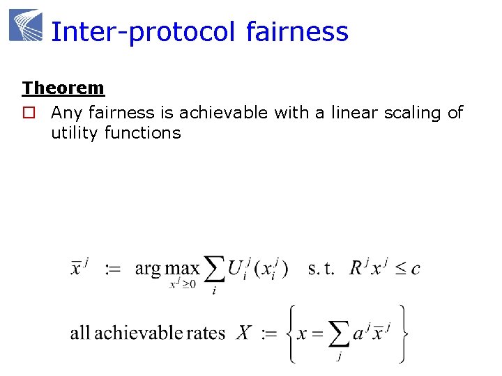
Inter-protocol fairness Theorem o Any fairness is achievable with a linear scaling of utility functions

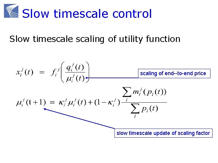
Slow timescale control Slow timescale scaling of utility function scaling of end--to-end price slow timescale update of scaling factor

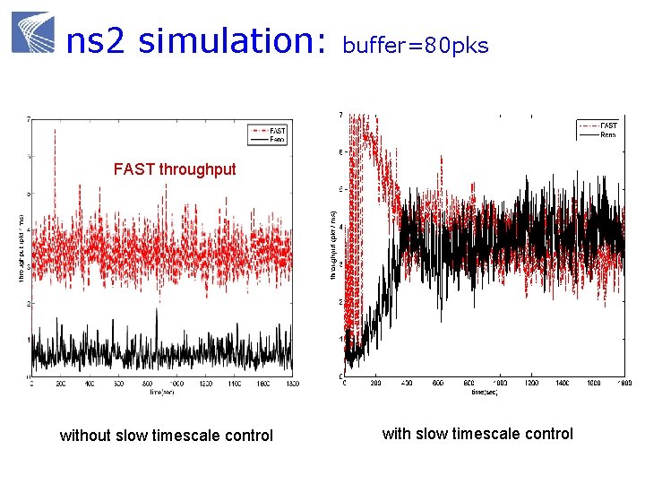
ns 2 simulation: buffer=80 pks FAST throughput without slow timescale control with slow timescale control

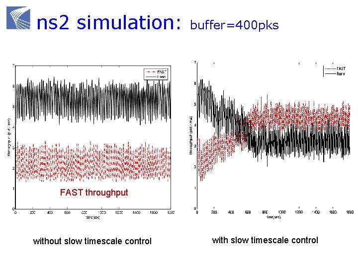
ns 2 simulation: buffer=400 pks FAST throughput without slow timescale control with slow timescale control

Advanced topics Heterogeneous protocols Layering as optimization decomposition

The Internet hourglass Applications Web Search Mail News Video Audio Friends TCP IP Ethernet 802. 11 3 G/4 G ATM Optical Link technologies Satellite Bluetooth

But what is architecture “Architecture involves or facilitates n n System-level function (beyond components) Organization and structure Protocols and modules Risk mitigation, performance, evolution but is more than the sum of these” -- John Doyle, Caltech “… the architecture of a system defines how the system is broken into parts and how those parts interact. ” -- Clark, Sollins, Wroclawski, …, MIT

But what is architecture “Things that persist over time” “Things that are common across networks” “Forms that enable functions” “Frozen but evolves” “It is intrinsic but artificial” Key features (John Doyle, Caltech) o Layering as optimization decomposition o Constraints that deconstrain o Robust yet fragile

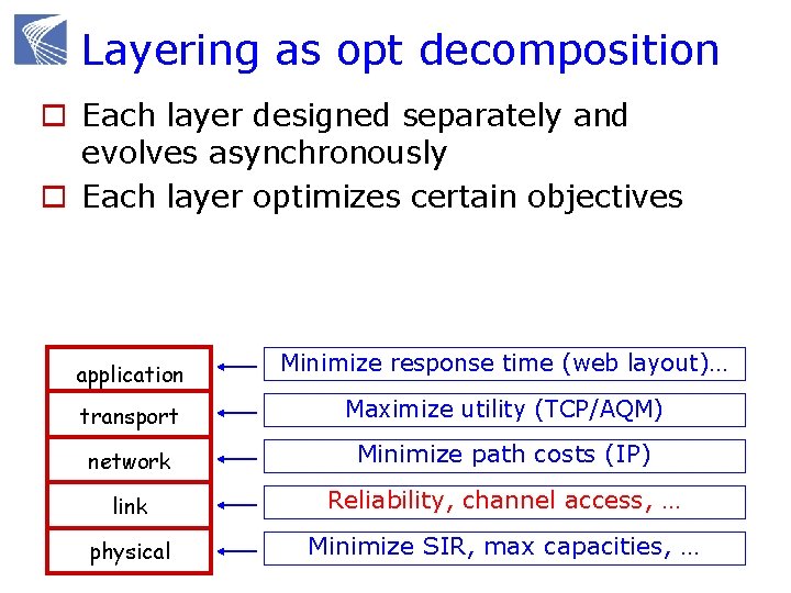
Layering as opt decomposition o Each layer designed separately and evolves asynchronously o Each layer optimizes certain objectives application Minimize response time (web layout)… transport Maximize utility (TCP/AQM) network Minimize path costs (IP) link Reliability, channel access, … physical Minimize SIR, max capacities, …

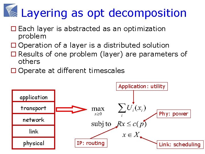
Layering as opt decomposition o Each layer is abstracted as an optimization problem o Operation of a layer is a distributed solution o Results of one problem (layer) are parameters of others o Operate at different timescales Application: utility application transport Phy: power network link physical IP: routing Link: scheduling

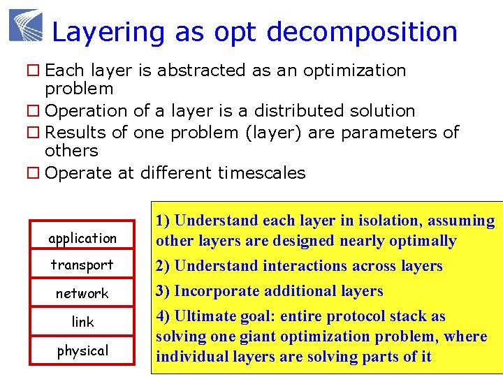
Layering as opt decomposition o Each layer is abstracted as an optimization problem o Operation of a layer is a distributed solution o Results of one problem (layer) are parameters of others o Operate at different timescales application transport network link physical 1) Understand each layer in isolation, assuming other layers are designed nearly optimally 2) Understand interactions across layers 3) Incorporate additional layers 4) Ultimate goal: entire protocol stack as solving one giant optimization problem, where individual layers are solving parts of it

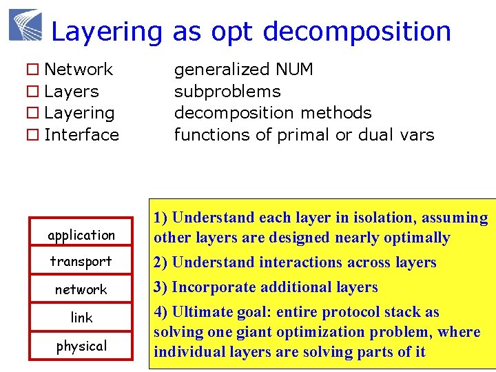
Layering as opt decomposition o Network o Layers o Layering o Interface application transport network link physical generalized NUM subproblems decomposition methods functions of primal or dual vars 1) Understand each layer in isolation, assuming other layers are designed nearly optimally 2) Understand interactions across layers 3) Incorporate additional layers 4) Ultimate goal: entire protocol stack as solving one giant optimization problem, where individual layers are solving parts of it

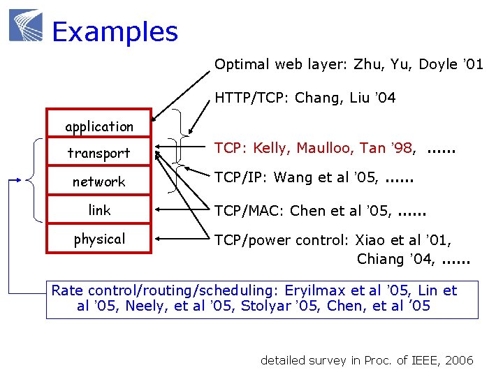
Examples Optimal web layer: Zhu, Yu, Doyle ’ 01 HTTP/TCP: Chang, Liu ’ 04 application transport network link physical TCP: Kelly, Maulloo, Tan ’ 98, …… TCP/IP: Wang et al ’ 05, …… TCP/MAC: Chen et al ’ 05, …… TCP/power control: Xiao et al ’ 01, Chiang ’ 04, …… Rate control/routing/scheduling: Eryilmax et al ’ 05, Lin et al ’ 05, Neely, et al ’ 05, Stolyar ’ 05, Chen, et al ’ 05 detailed survey in Proc. of IEEE, 2006

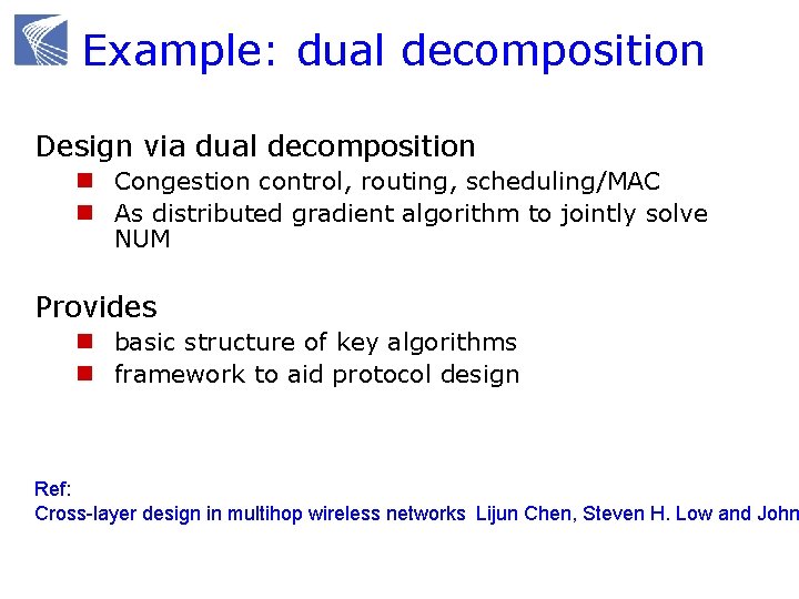
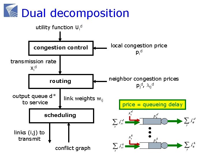
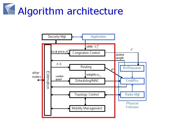
Example: dual decomposition Design via dual decomposition n Congestion control, routing, scheduling/MAC n As distributed gradient algorithm to jointly solve NUM Provides n basic structure of key algorithms n framework to aid protocol design Ref: Cross-layer design in multihop wireless networks
Lijun Chen, Steven H. Low and John

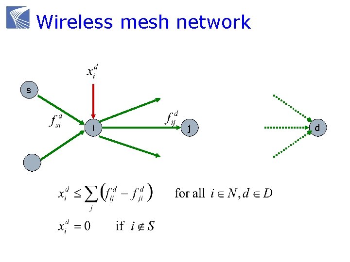
Wireless mesh network s i j d

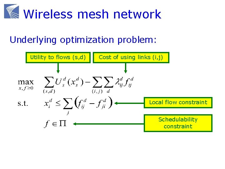
Wireless mesh network Underlying optimization problem: Utility to flows (s, d) Cost of using links (i, j) Local flow constraint Schedulability constraint

Dual decomposition utility function Uid congestion control local congestion price pid transmission rate xid routing output queue d* to service link weights wij scheduling links (i, j) to transmit conflict graph neighbor congestion prices pjd, lijd price = queueing delay

Algorithm architecture Security Mgt Application utility local price Congestion Control Routing Estimation other nodes conflict graph queue length d* En/Dequeue weights Scheduling/MAC Xmit/Rcv Topology Control Radio Mgt Mobility Management Physical Xmission