Congestion Control In The Internet JY Le Boudec

Congestion Control In The Internet JY Le Boudec Fall 2009 1

Plan of This Module 1. Congestion control: theory 2. Application to the Internet 2

Theory of Congestion Control What you have to learn in this first part: 1. What is the problem; congestion collapse 2. Efficiency versus Fairness 3. Forms of fairness 4. Forms of congestion control 5. Additive Increase Multiplicative Decrease (AIMD) 3

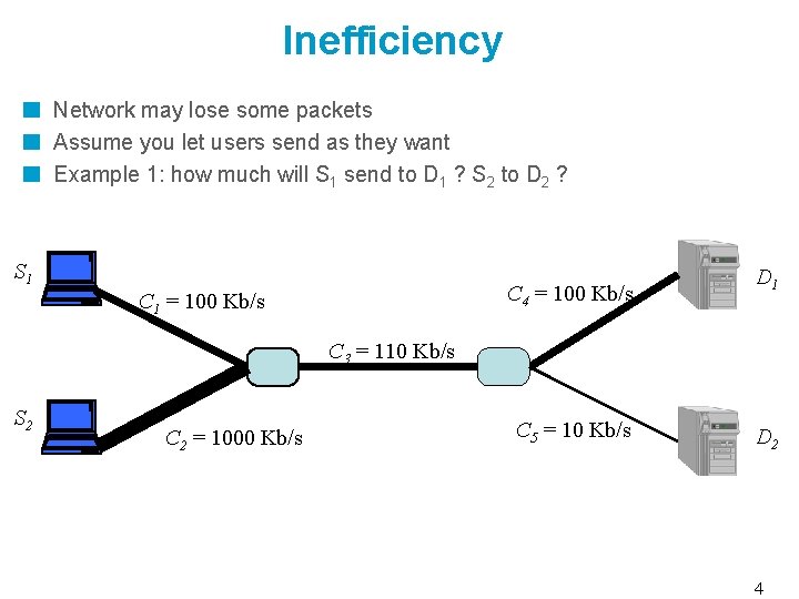
Inefficiency Network may lose some packets Assume you let users send as they want Example 1: how much will S 1 send to D 1 ? S 2 to D 2 ? S 1 C 4 = 100 Kb/s C 1 = 100 Kb/s D 1 C 3 = 110 Kb/s S 2 C 2 = 1000 Kb/s C 5 = 10 Kb/s D 2 4

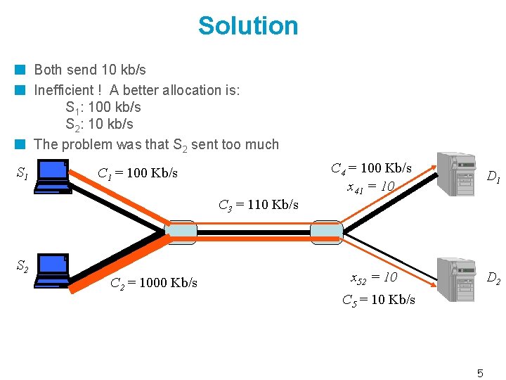
Solution Both send 10 kb/s Inefficient ! A better allocation is: S 1: 100 kb/s S 2: 10 kb/s The problem was that S 2 sent too much S 1 C 1 = 100 Kb/s C 4 = 100 Kb/s x 41 = 10 D 1 x 52 = 10 D 2 C 3 = 110 Kb/s S 2 C 2 = 1000 Kb/s C 5 = 10 Kb/s 5

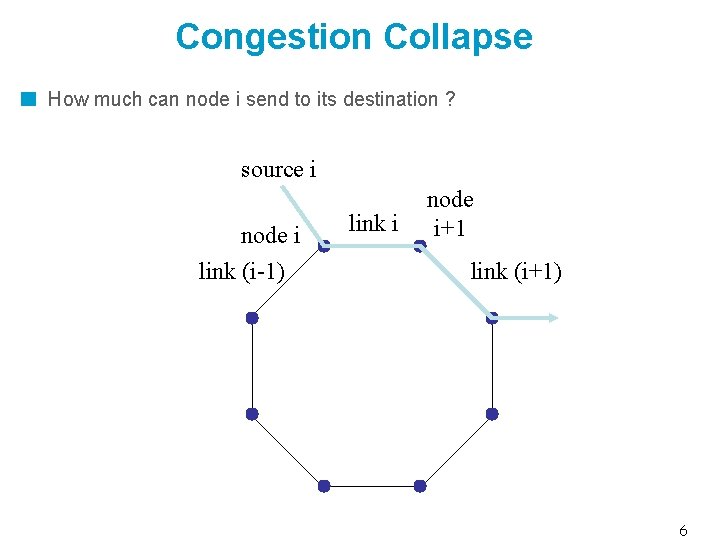
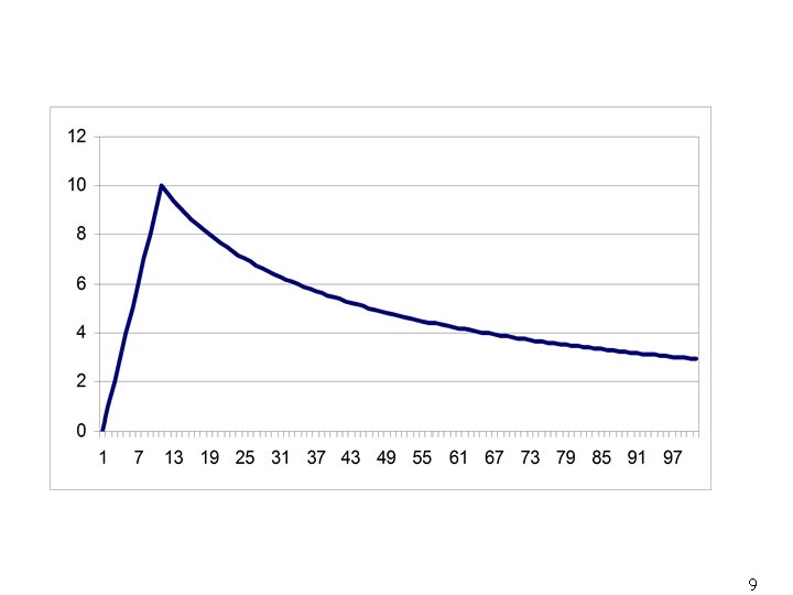
Congestion Collapse How much can node i send to its destination ? source i node i link (i-1) link i node i+1 link (i+1) 6

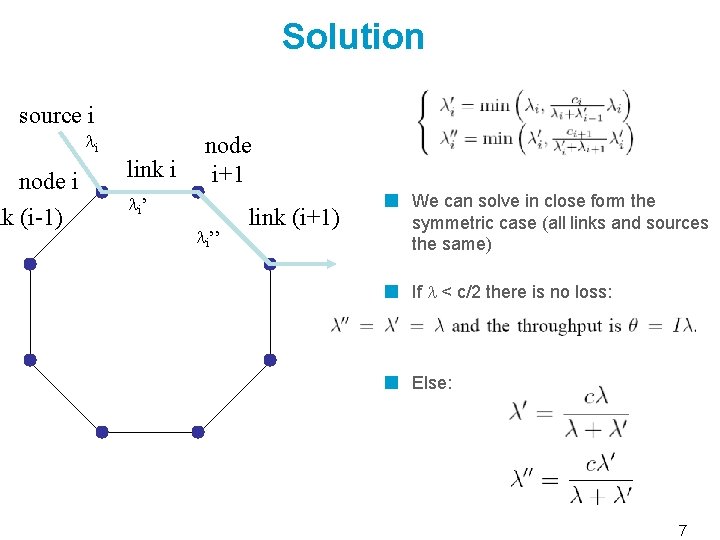
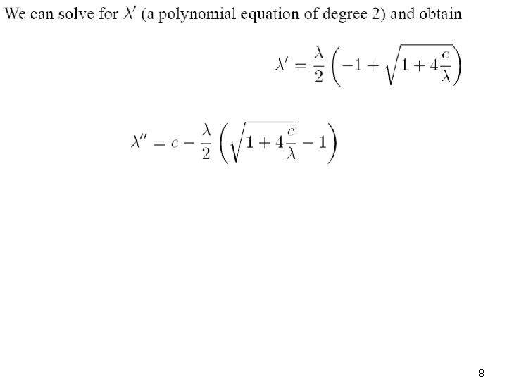
Solution source i node i nk (i-1) i link i node i+1 i’ i’’ link (i+1) We can solve in close form the symmetric case (all links and sources the same) If < c/2 there is no loss: Else: 7

8

9

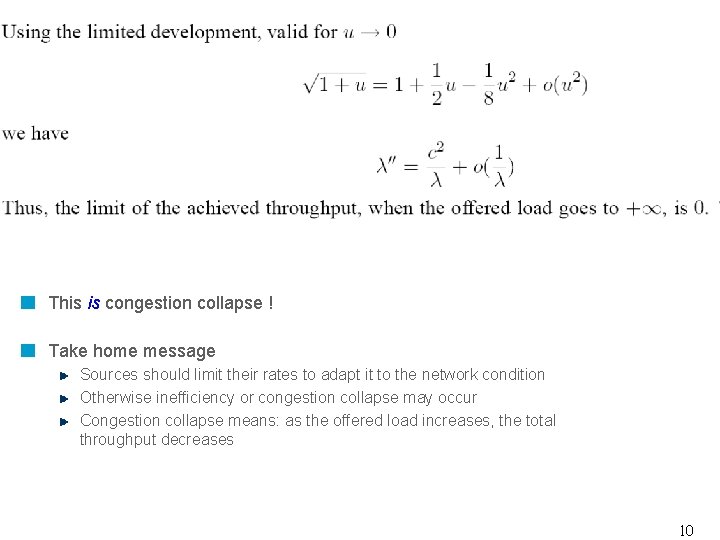
This is congestion collapse ! Take home message Sources should limit their rates to adapt it to the network condition Otherwise inefficiency or congestion collapse may occur Congestion collapse means: as the offered load increases, the total throughput decreases 10

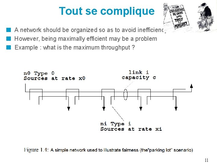
Tout se complique A network should be organized so as to avoid inefficiency However, being maximally efficient may be a problem Example : what is the maximum throughput ? 11

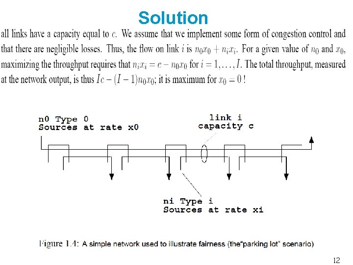
Solution 12

Take Home Message Efficiency may be at the expense of fairness What is fairness ? 13

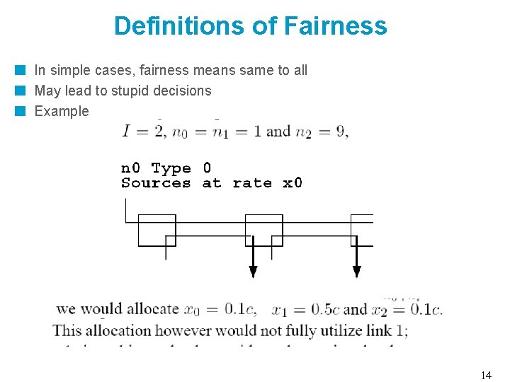
Definitions of Fairness In simple cases, fairness means same to all May lead to stupid decisions Example 14

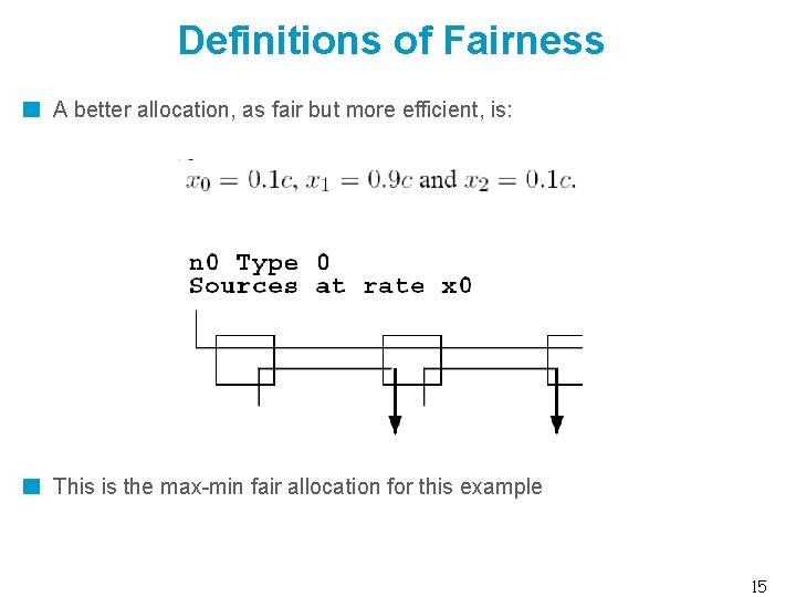
Definitions of Fairness A better allocation, as fair but more efficient, is: This is the max-min fair allocation for this example 15

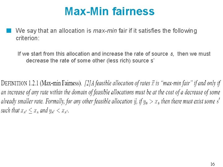
Max-Min fairness We say that an allocation is max-min fair if it satisfies the following criterion: If we start from this allocation and increase the rate of source s, then we must decrease the rate of some other (less rich) source s’ 16

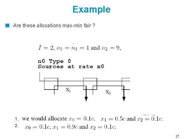
Example Are these allocations max-min fair ? X 1 X 2 1. 2. 17

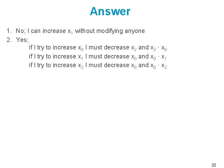
Answer 1. No; I can increase x 1 without modifying anyone 2. Yes; if I try to increase x 0 I must decrease x 2 and x 2 · x 0 if I try to increase x 1 I must decrease x 0 and x 0 · x 1 if I try to increase x 2 I must decrease x 0 and x 0 · x 2 18

The Maths of Max-Min Fairness Given a set of constraints for the rates If it exists, the max-min fair allocation is unique There exists one max-min fair allocation if the set of feasible rates is convex (this is the case for networks, we have linear constraints) For a set of feasible rates as in our case (the sum of the rates on every link is upper bounded), the (unique) max min fair allocation is obtained by water-filling 19

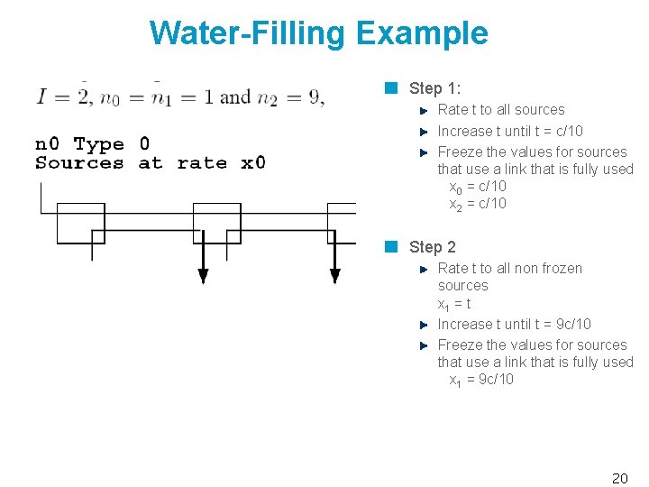
Water-Filling Example Step 1: Rate t to all sources Increase t until t = c/10 Freeze the values for sources that use a link that is fully used x 0 = c/10 x 2 = c/10 Step 2 Rate t to all non frozen sources x 1 = t Increase t until t = 9 c/10 Freeze the values for sources that use a link that is fully used x 1 = 9 c/10 20

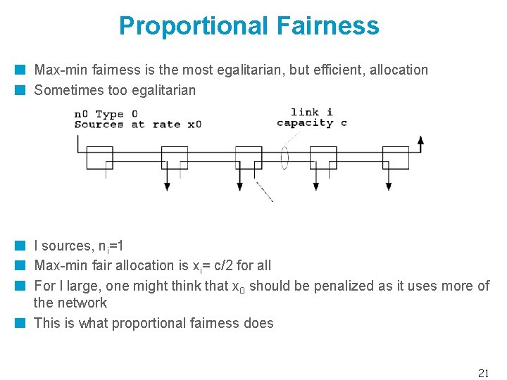
Proportional Fairness Max-min fairness is the most egalitarian, but efficient, allocation Sometimes too egalitarian I sources, ni=1 Max-min fair allocation is xi= c/2 for all For I large, one might think that x 0 should be penalized as it uses more of the network This is what proportional fairness does 21

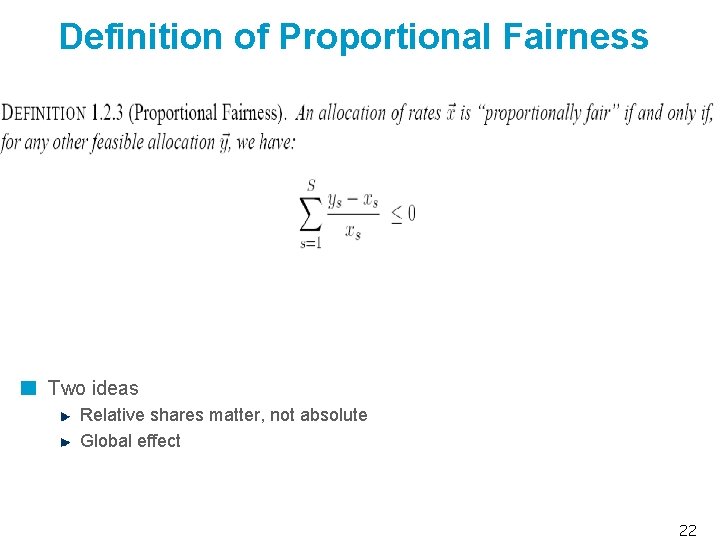
Definition of Proportional Fairness Two ideas Relative shares matter, not absolute Global effect 22

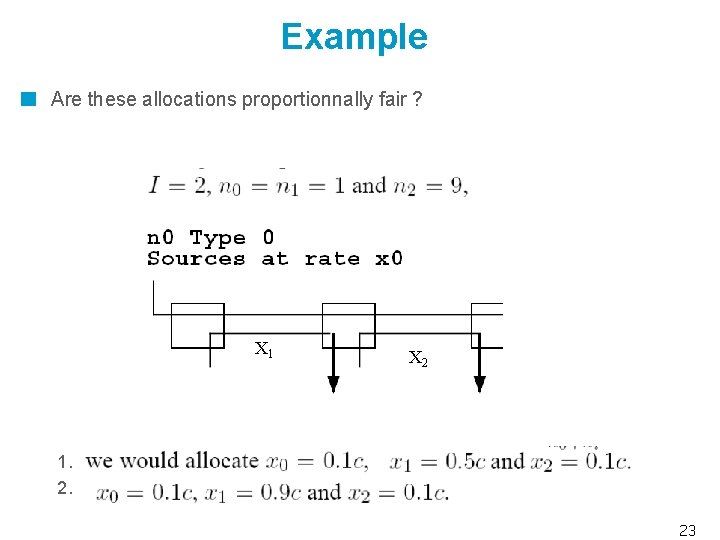
Example Are these allocations proportionnally fair ? X 1 X 2 1. 2. 23

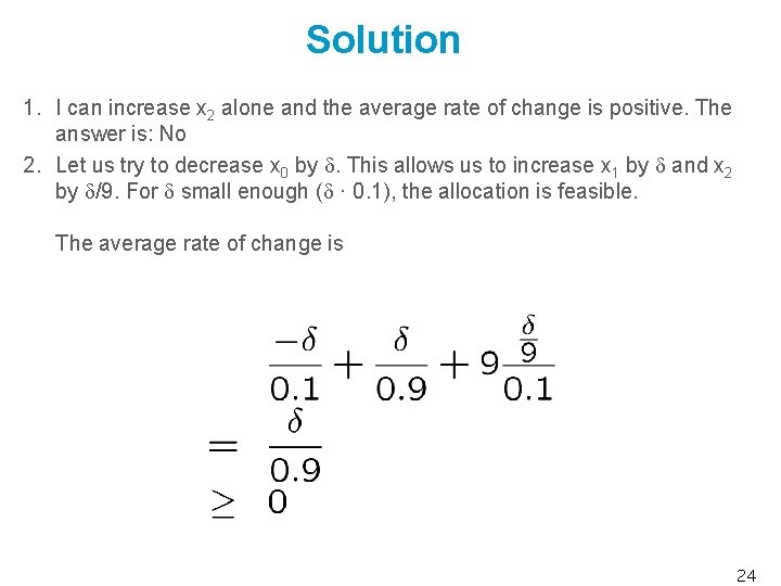
Solution 1. I can increase x 2 alone and the average rate of change is positive. The answer is: No 2. Let us try to decrease x 0 by . This allows us to increase x 1 by and x 2 by /9. For small enough ( · 0. 1), the allocation is feasible. The average rate of change is 24

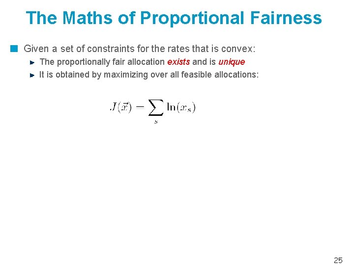
The Maths of Proportional Fairness Given a set of constraints for the rates that is convex: The proportionally fair allocation exists and is unique It is obtained by maximizing over all feasible allocations: 25

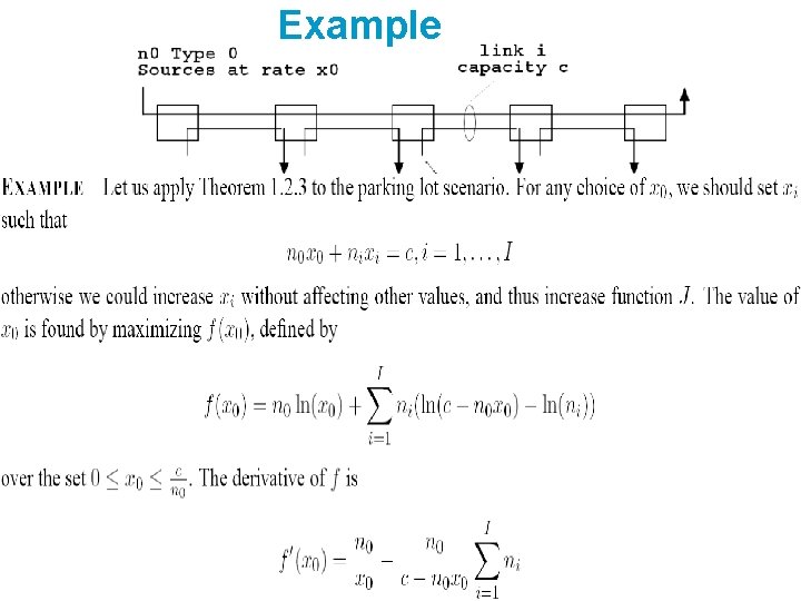
Example 26

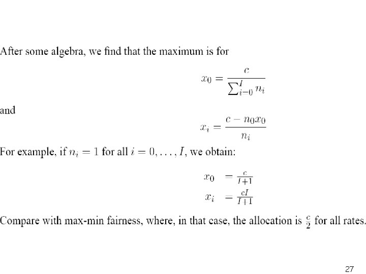
27

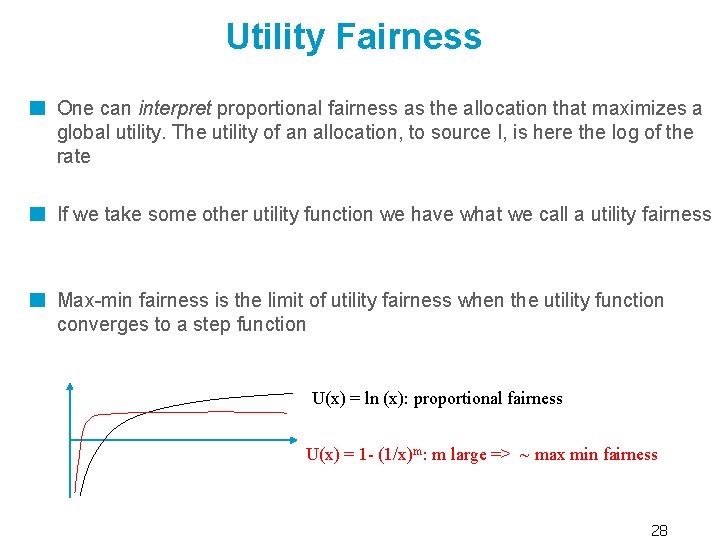
Utility Fairness One can interpret proportional fairness as the allocation that maximizes a global utility. The utility of an allocation, to source I, is here the log of the rate If we take some other utility function we have what we call a utility fairness Max-min fairness is the limit of utility fairness when the utility function converges to a step function U(x) = ln (x): proportional fairness U(x) = 1 - (1/x)m: m large => ~ max min fairness 28

Take Home Message Sources should adapt their rate to the state of the network in order to avoid inefficiencies and congestion collapse This is called “congestion control” A rate adaptation mechanism should target some form of fairness E. g. max-min fairness or proportional fairness 29

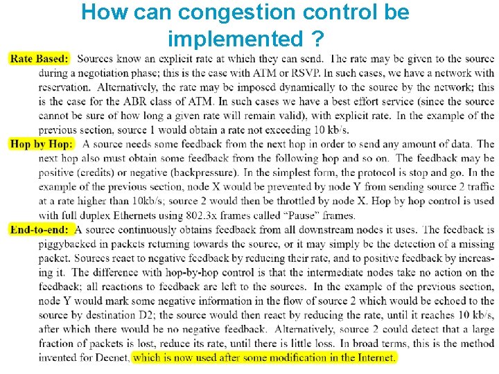
How can congestion control be implemented ? 30

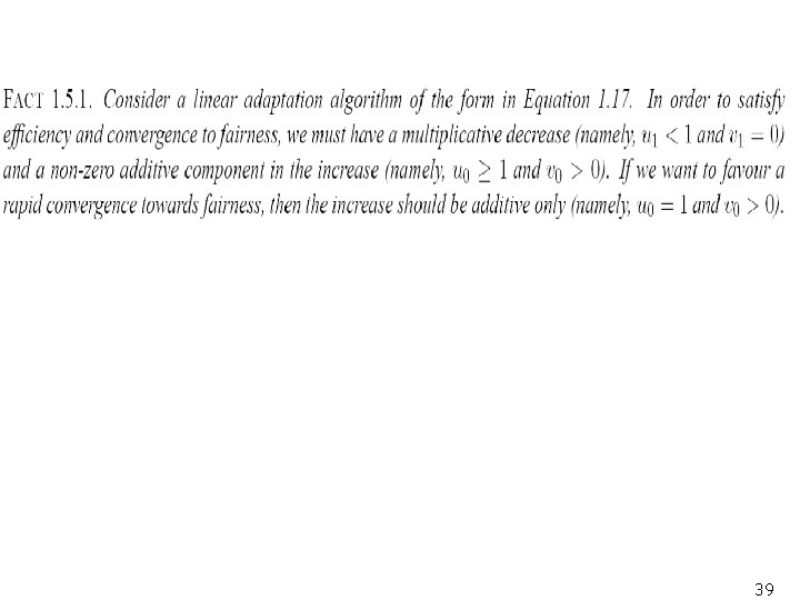
Additive Increase Multiplicative Decrease It is a congestion control mechanism that can be implemented end to end It is the basis for what we have in the Internet We explain it on a simple example 31

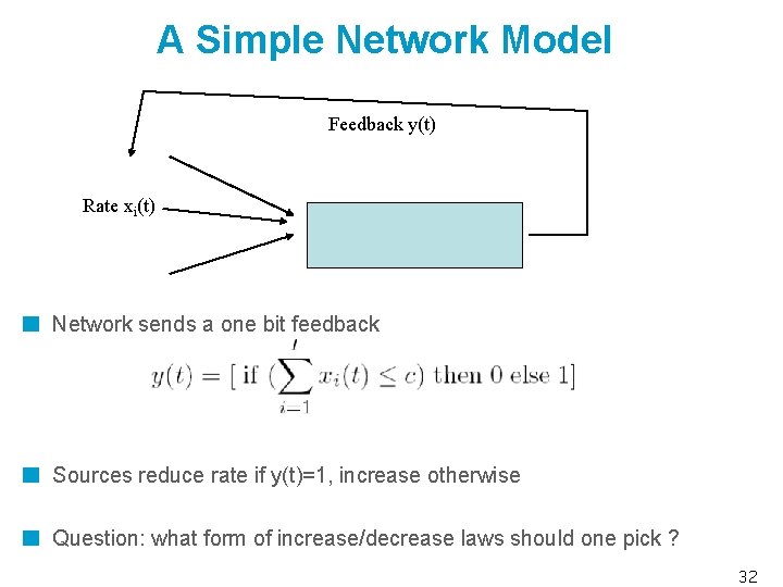
A Simple Network Model Feedback y(t) Rate xi(t) Network sends a one bit feedback Sources reduce rate if y(t)=1, increase otherwise Question: what form of increase/decrease laws should one pick ? 32

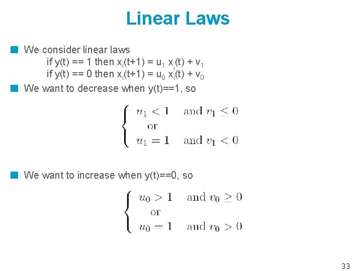
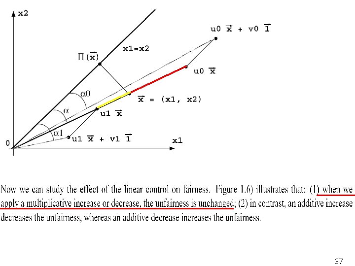
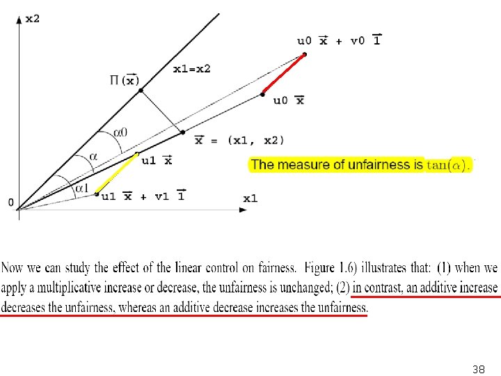
Linear Laws We consider linear laws if y(t) == 1 then xi(t+1) = u 1 xi(t) + v 1 if y(t) == 0 then xi(t+1) = u 0 xi(t) + v 0 We want to decrease when y(t)==1, so We want to increase when y(t)==0, so 33

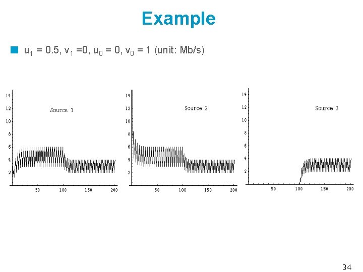
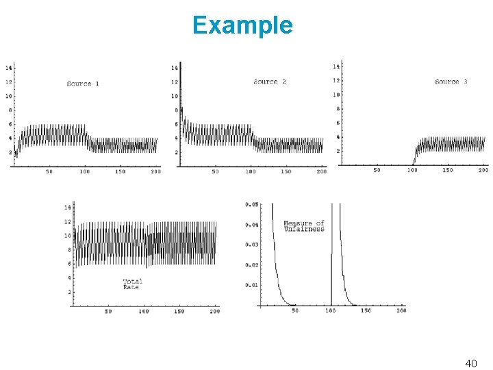
Example u 1 = 0. 5, v 1 =0, u 0 = 0, v 0 = 1 (unit: Mb/s) 34

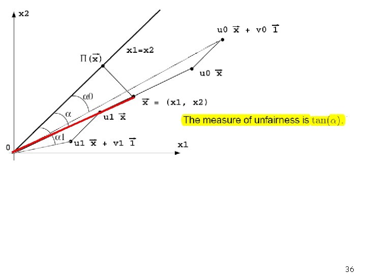
Impact of Fairness Does such a scheme converge to a fair allocation ? Here max-min and proportionally fair are the same (i. e. same rate to all) The scheme may not converge as sources may not be stationary But we would like that the scheme increases fairness 35

36

37

38

39

Example 40

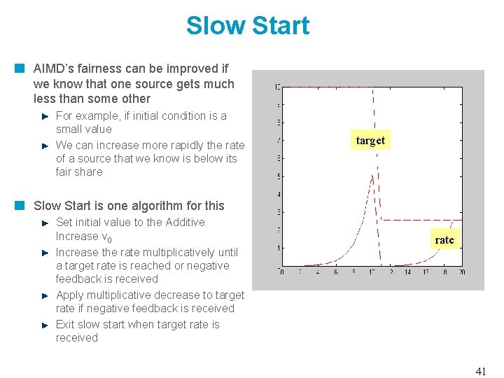
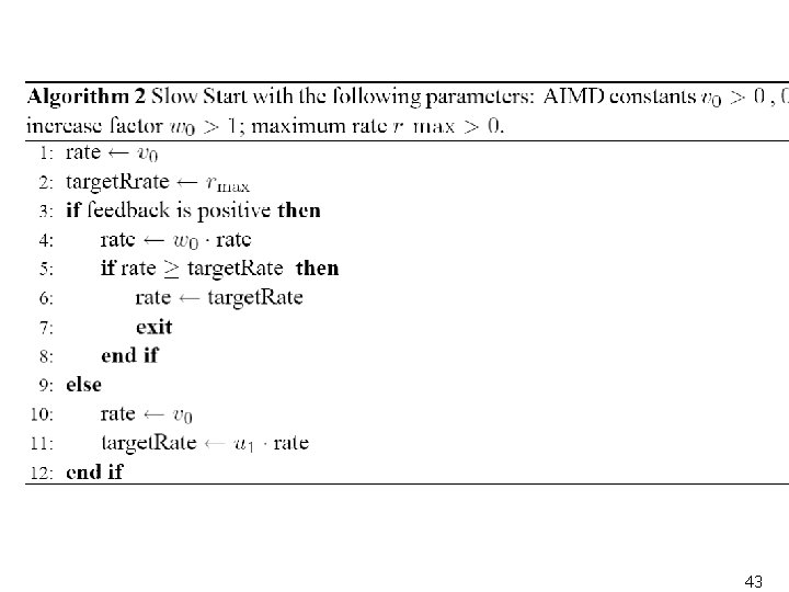
Slow Start AIMD’s fairness can be improved if we know that one source gets much less than some other For example, if initial condition is a small value We can increase more rapidly the rate of a source that we know is below its fair share target Slow Start is one algorithm for this Set initial value to the Additive Increase v 0 Increase the rate multiplicatively until a target rate is reached or negative feedback is received Apply multiplicative decrease to target rate if negative feedback is received Exit slow start when target rate is received rate 41

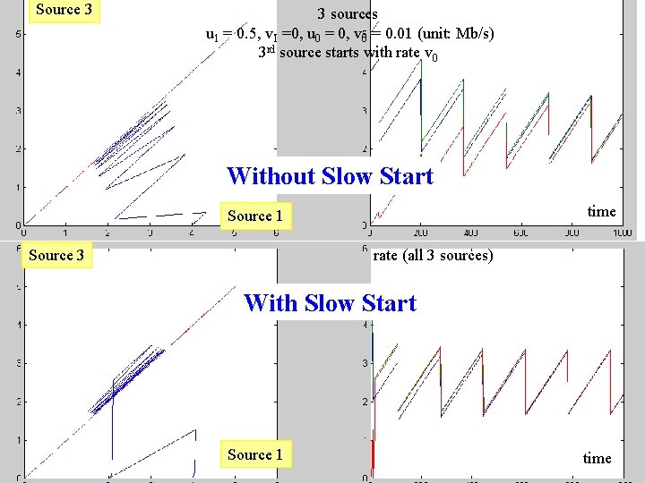
Source 3 3 sources u 1 = 0. 5, v 1 =0, u 0 = 0, v 0 = 0. 01 (unit: Mb/s) 3 rd source starts with rate v 0 Without Slow Start time Source 1 Source 3 rate (all 3 sources) With Slow Start Source 1 time 42

43

Plan of This Module 1. Congestion control: theory 2. Application to the Internet 44

Congestion Control in the Internet is in TCP is used to avoid congestion in the Internet in addition to what was shown: a TCP source adjusts its window to the congestion status of the Internet (slow start, congestion avoidance) this avoids congestion collapse and ensures some fairness TCP sources interprets losses as a negative feedback use to reduce the sending rate UDP sources are a problem for the Internet use for long lived sessions (ex: Real. Audio) is a threat: congestion collapse UDP sources should imitate TCP : “TCP friendly” 45

TCP Congestion Control is based on AIMD TCP adjusts the window size (in addition to offered window ie credit mechanism) W = min (cwnd, Offered. Window) Principles of TCP Congestion Control negative feedback = loss, positive feedback = ACK received Additive Increase (1 MSS), Multiplicative Decrease (0. 5) Slow start with increase factor = 2 Reaction to loss depends on nature of loss detection Loss detected by timeout => slow start Loss detected by fast retransmit or selective Ack => no slow start 46

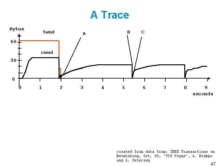
A Trace Bytes twnd B A C 60 cwnd 30 0 0 1 2 3 4 5 6 7 8 9 seconds created from data from: IEEE Transactions on Networking, Oct. 95, “TCP Vegas”, L. Brakmo and L. Petersen 47

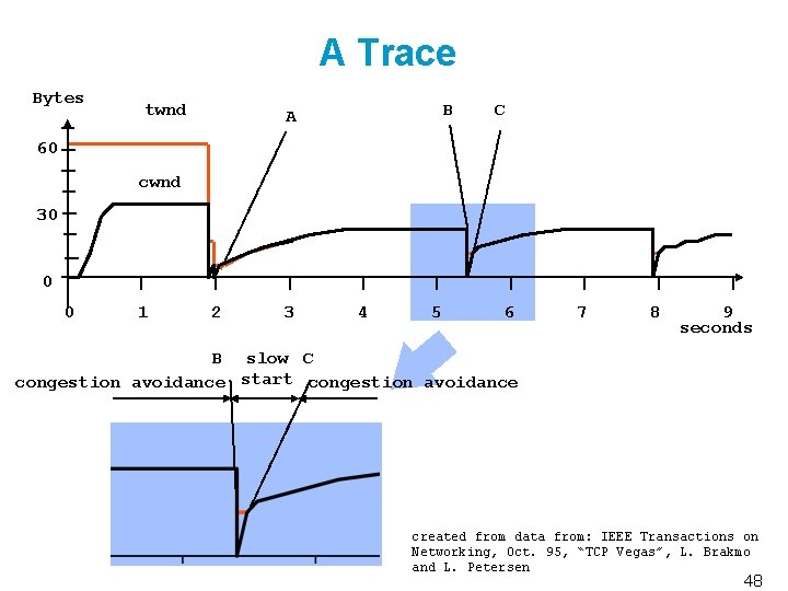
A Trace Bytes twnd B A C 60 cwnd 30 0 0 1 2 3 4 5 6 7 8 9 seconds B slow C congestion avoidance start congestion avoidance created from data from: IEEE Transactions on Networking, Oct. 95, “TCP Vegas”, L. Brakmo and L. Petersen 48

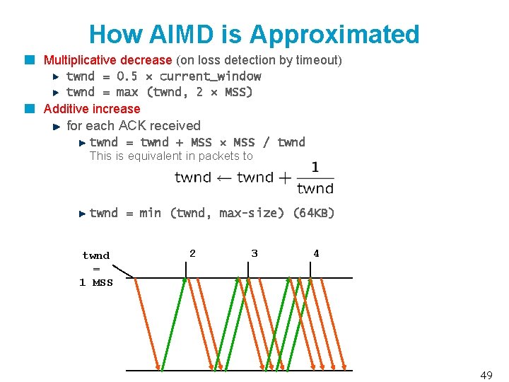
How AIMD is Approximated Multiplicative decrease (on loss detection by timeout) twnd = 0. 5 current_window twnd = max (twnd, 2 MSS) Additive increase for each ACK received twnd = twnd + MSS / twnd This is equivalent in packets to twnd = min (twnd, max-size) (64 KB) twnd = 1 MSS 2 3 4 49

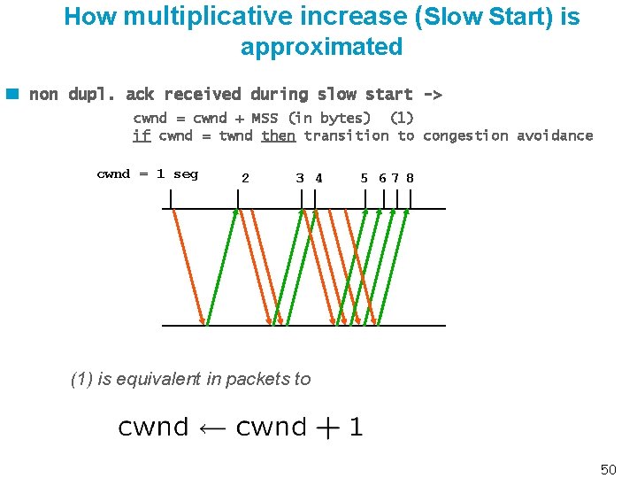
How multiplicative increase (Slow Start) is approximated non dupl. ack received during slow start -> cwnd = cwnd + MSS (in bytes) (1) if cwnd = twnd then transition to congestion avoidance cwnd = 1 seg 2 3 4 5 678 (1) is equivalent in packets to 50

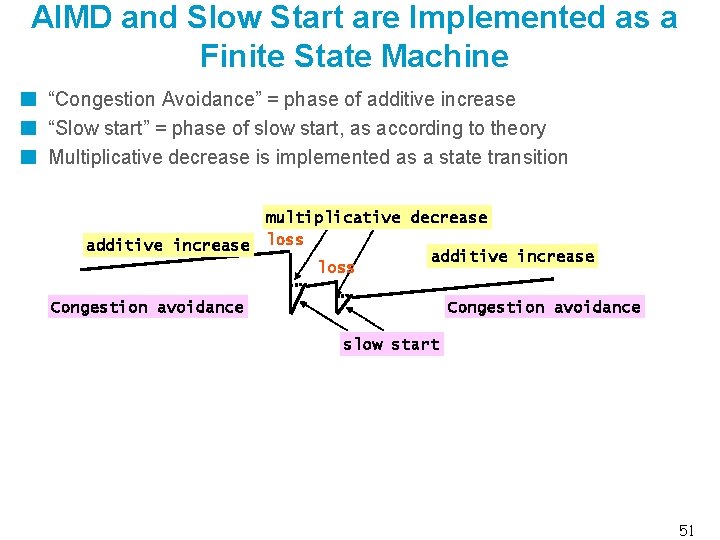
AIMD and Slow Start are Implemented as a Finite State Machine “Congestion Avoidance” = phase of additive increase “Slow start” = phase of slow start, as according to theory Multiplicative decrease is implemented as a state transition additive increase multiplicative decrease loss additive increase loss Congestion avoidance slow start 51

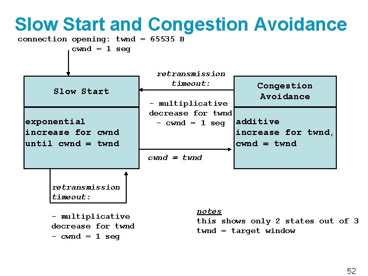
Slow Start and Congestion Avoidance connection opening: twnd = 65535 B cwnd = 1 seg Slow Start exponential increase for cwnd until cwnd = twnd retransmission timeout: Congestion Avoidance - multiplicative decrease for twnd - cwnd = 1 seg additive increase for twnd, cwnd = twnd retransmission timeout: - multiplicative decrease for twnd - cwnd = 1 seg notes this shows only 2 states out of 3 twnd = target window 52

Fast Recovery Slow start used when we assume that the network condition is new initial phase, major change guessed by timeout expiration In all other packet loss detection events, slow start is not used, but “fast recovery” is used instead target window is halved but temporary window size increase is allowed to help recover losses when a loss occurs, the sending rate is no longer approximated by the W/RTT 53

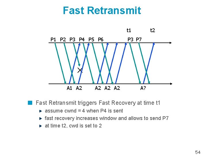
Fast Retransmit t 1 P 2 P 3 P 4 P 5 P 6 t 2 P 3 P 7 A 1 A 2 A 2 A? Fast Retransmit triggers Fast Recovery at time t 1 assume cwnd = 4 when P 4 is sent fast recovery increases window and allows to send P 7 at time t 2, cwd is set to 2 54

Fast Recovery Details Multiplicative decrease twnd = 0. 5 current-size twnd = max (twnd, 2 MSS) Fast Recovery cwnd = twnd + 3 MSS (exp. increase) cwnd = min (cwnd, 64 K) retransmission of the missing segment (n) For each duplicated ACK cwnd = cwnd + MSS (exp. increase) cwnd = min (cwnd, 64 K) send following segments 55

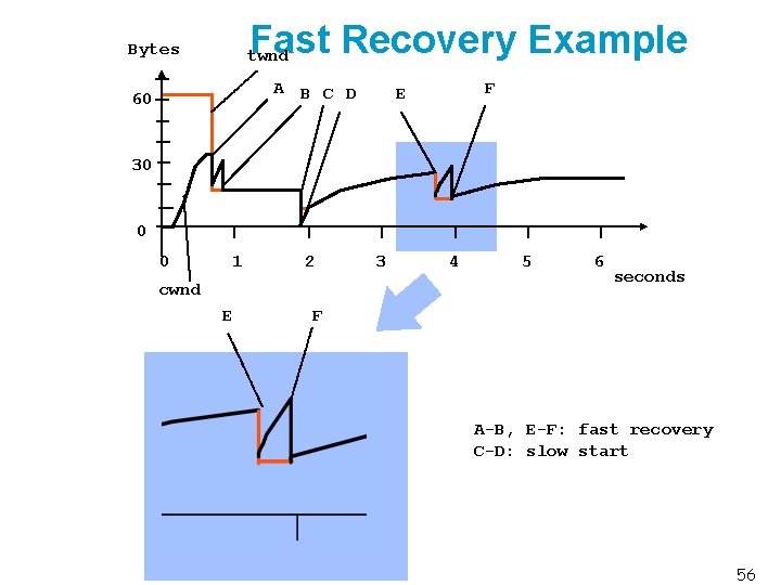
Fast Recovery Example Bytes twnd A 60 B C D F E 30 0 0 1 2 cwnd E 3 4 5 6 seconds F A-B, E-F: fast recovery C-D: slow start 56

TCP Congestion Control Has Three States new connection: cwnd = twnd: Slow Start - exponential increase retr. timeout: fast retransmit: Congestion Avoidance - additive increase fast retransmit: retr. timeout: Fast Recovery retr. timeout: - exponential increase beyond twnd expected ack received: 57

Fairness of TCP implements some approximation of AIMD is designed to be approximately fair in a single link scenario Q: what happens in a network ? Does TCP distribute rates according to max-min fairness or proportional fairness ? 58

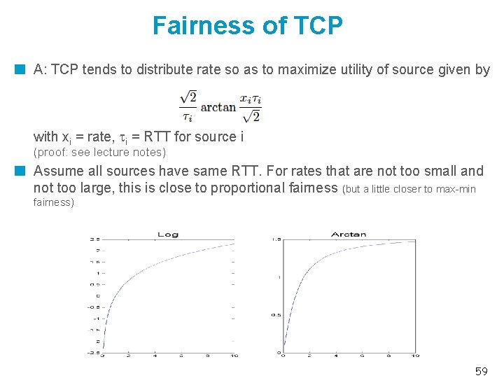
Fairness of TCP A: TCP tends to distribute rate so as to maximize utility of source given by with xi = rate, i = RTT for source i (proof: see lecture notes) Assume all sources have same RTT. For rates that are not too small and not too large, this is close to proportional fairness (but a little closer to max-min fairness) 59

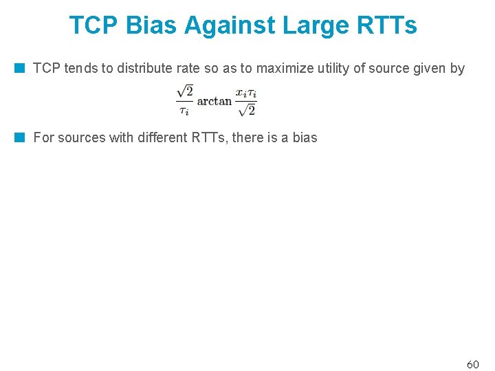
TCP Bias Against Large RTTs TCP tends to distribute rate so as to maximize utility of source given by For sources with different RTTs, there is a bias 60

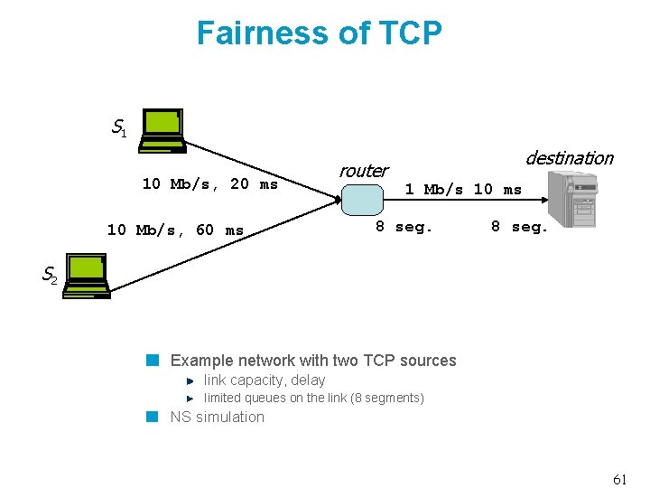
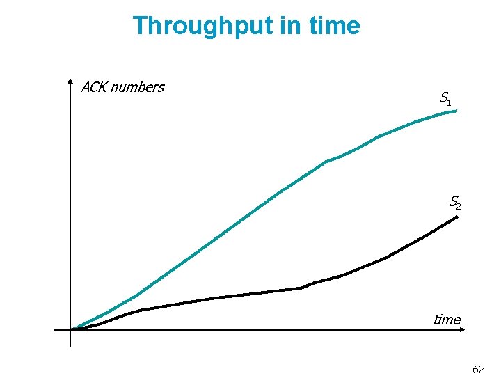
Fairness of TCP S 1 10 Mb/s, 20 ms 10 Mb/s, 60 ms router destination 1 Mb/s 10 ms 8 seg. S 2 Example network with two TCP sources link capacity, delay limited queues on the link (8 segments) NS simulation 61

Throughput in time ACK numbers S 1 S 2 time 62

Bias of TCP Against Large RTTs A source that uses many hops obtains less because it uses more resources (¼ proportional fairness) – desired bias it has a longer RTT – undesired bias Cause is additive increase is one packet per RTT 63

AQM By default. routers drop packets when buffers are full this is called “Tail Drop” Issues buffers fill, then drop -> buffers are full most of the time produces large average delays large queuing delay => large RTT => smaller TCP throughput also: produces very irregular behaviour but buffers are needed to amortize bursts Solution active queue management (AQM) drop packets before buffer is full, based on estimation of traffic load 64

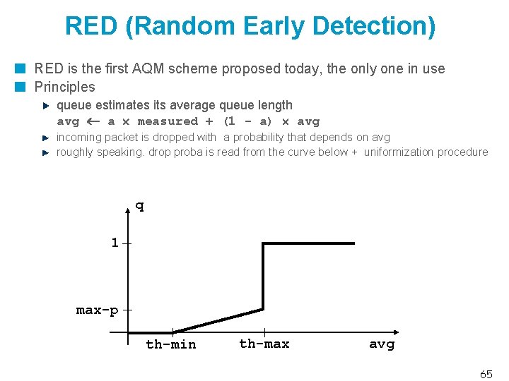
RED (Random Early Detection) RED is the first AQM scheme proposed today, the only one in use Principles queue estimates its average queue length avg a measured + (1 - a) avg incoming packet is dropped with a probability that depends on avg roughly speaking. drop proba is read from the curve below + uniformization procedure q 1 max-p th-min th-max avg 65

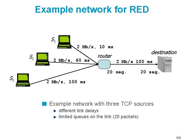
Example network for RED S 1 2 Mb/s, 10 ms S 2 S 3 2 Mb/s, 60 ms destination router 2 Mb/s 100 ms 20 seg. 2 Mb/s, 100 ms Example network with three TCP sources different link delays limited queues on the link (20 packets) 66

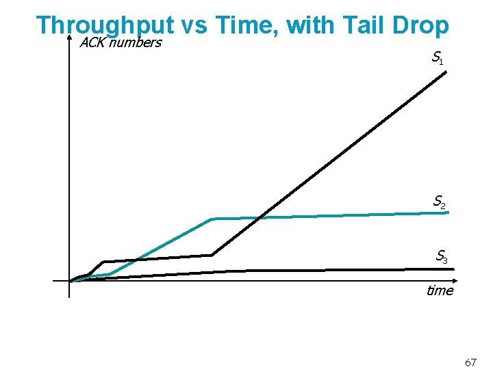
Throughput vs Time, with Tail Drop ACK numbers S 1 S 2 S 3 time 67

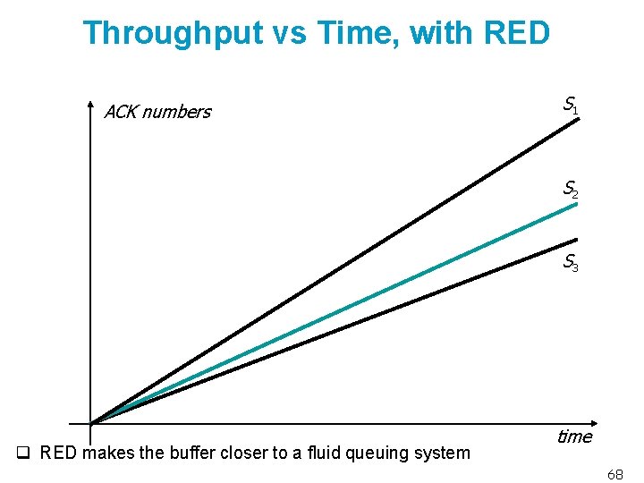
Throughput vs Time, with RED ACK numbers S 1 S 2 S 3 q RED makes the buffer closer to a fluid queuing system time 68

TCP Loss - Throughput Formula Consider a large TCP connection (many bytes to transmit) Assume we observe that, in average, a fraction q of packets is lost (or marked with ECN) Can we say something about the expected throughput for this connection ? 69

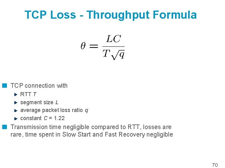
TCP Loss - Throughput Formula TCP connection with RTT T segment size L average packet loss ratio q constant C = 1. 22 Transmission time negligible compared to RTT, losses are rare, time spent in Slow Start and Fast Recovery negligible 70

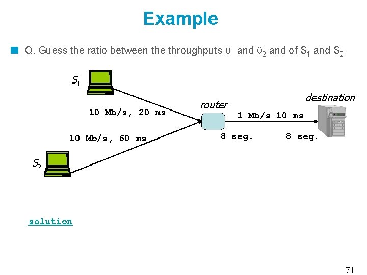
Example Q. Guess the ratio between the throughputs 1 and 2 and of S 1 and S 2 S 1 10 Mb/s, 20 ms 10 Mb/s, 60 ms router destination 1 Mb/s 10 ms 8 seg. S 2 solution 71

TCP Friendly Applications All TCP/IP applications that generate long lived flows should mimic the behavior of a TCP source RTP/UDP flow sending video/audio data Adaptive algorithm application determines the sending rate feedback - amount of lost packets, loss ratio sending rate = rate of a TCP flow experiencing the same loss ratio 72

Facts to remember TCP performs congestion control in end-systems sender increases its sending window until loss occurs, then decreases additive increase (no loss) multiplicative decrease (loss) TCP states slow start, congestion avoidance, fast recovery Negative bias towards long round trip times UDP applications should behave like TCP with the same loss rate 73

Congestion Control: Summary Congestion control aims at avoiding congestion collapse in the network With TCP/IP, performed in end-systems, mainly with TCP Congestion control summary Principle: sender increases its sending window until losses occur, then decrease additive increase multiplicative decrease loss additive increase loss slow start target window: additive increase (no loss), multiplicative decrease (loss) 3 phases: slow start: starts with 1, exponential increase up to twnd congestion avoidance: additive increase until loss or no increase fast recovery: fast retransmission of one segment slow start entered at setup or after retransmission timeout fast recovery entered at fast retransmit 74

Solutions 75

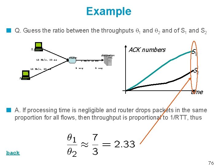
Example Q. Guess the ratio between the throughputs 1 and 2 and of S 1 and S 2 ACK numbers S 1 10 Mb/s, 20 ms 10 Mb/s, 60 ms destination router S 1 1 Mb/s 10 ms 8 seg. S 2 time A. If processing time is negligible and router drops packets in the same proportion for all flows, then throughput is proportional to 1/RTT, thus back 76