Confirmatory Factor Analysis in R with lavaan OARC

Confirmatory Factor Analysis in R with lavaan OARC IDRE Statistical Consulting https: //stats. idre. ucla. edu/r/seminars/rcfa/ 1

Outline 1 • Introduction • • • Motivating example: The SAQ Variance-covariance matrix Factor analysis model Model-implied covariance matrix Path Diagram • One Factor CFA • • Known values, parameters, and degrees of freedom Three-item (one) factor analysis Identification of a three-item one factor CFA Running a one-factor CFA in lavaan 2

Outline 2 • Model Fit Statistics • Model chi-square • Approximate fit indices • CFI (Confirmatory Factor Index) • TLI (Tucker Lewis Index) • RMSEA • Two Factor Confirmatory Factor Analysis • Correlated factors • Intermission • Exercises 3

Introduction • • • Motivating example: The SAQ Variance-covariance matrix Factor analysis model Model-implied covariance matrix Path Diagram 4

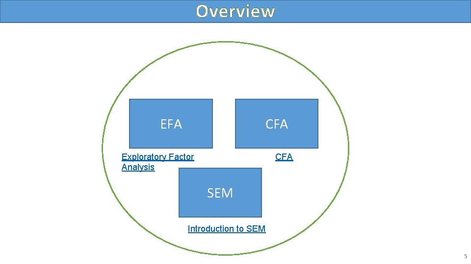
Overview EFA CFA Exploratory Factor Analysis CFA SEM Introduction to SEM 5

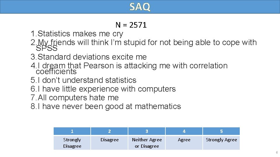
SAQ N = 2571 1. Statistics makes me cry 2. My friends will think I’m stupid for not being able to cope with SPSS 3. Standard deviations excite me 4. I dream that Pearson is attacking me with correlation coefficients 5. I don’t understand statistics 6. I have little experience with computers 7. All computers hate me 8. I have never been good at mathematics 1 2 3 4 5 Strongly Disagree Neither Agree or Disagree Agree Strongly Agree 6

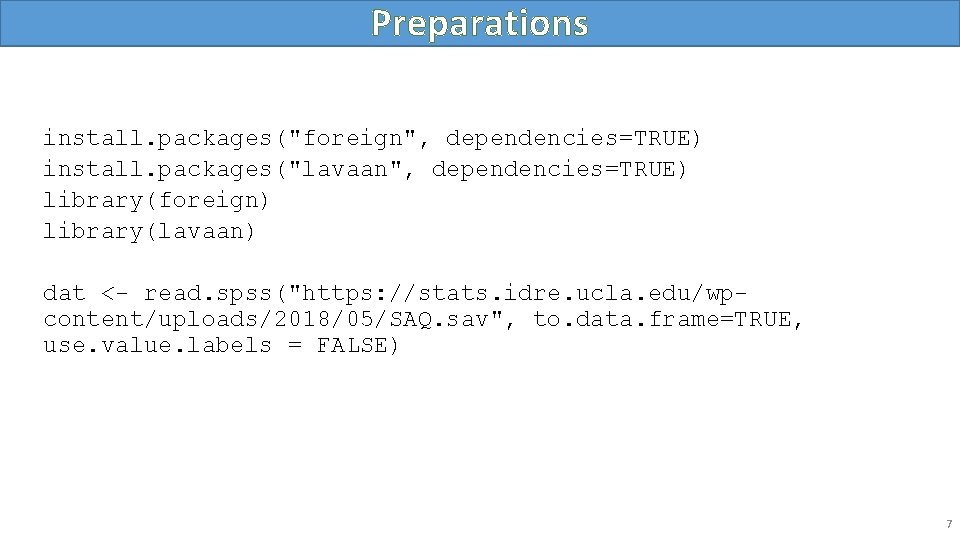
Preparations install. packages("foreign", dependencies=TRUE) install. packages("lavaan", dependencies=TRUE) library(foreign) library(lavaan) dat <- read. spss("https: //stats. idre. ucla. edu/wpcontent/uploads/2018/05/SAQ. sav", to. data. frame=TRUE, use. value. labels = FALSE) 7

Correlation Table > round(cor(dat[, 1: 8]), 2) q 01 q 02 q 03 q 04 q 05 q 06 q 07 q 08 q 01 1. 00 -0. 10 -0. 34 0. 40 0. 22 0. 31 0. 33 q 02 -0. 10 1. 00 0. 32 -0. 11 -0. 12 -0. 07 -0. 16 -0. 05 q 03 -0. 34 0. 32 1. 00 -0. 38 -0. 31 -0. 23 -0. 38 -0. 26 q 04 0. 44 -0. 11 -0. 38 1. 00 0. 40 0. 28 0. 41 0. 35 q 05 0. 40 -0. 12 -0. 31 0. 40 1. 00 0. 26 0. 34 0. 27 q 06 0. 22 -0. 07 -0. 23 0. 28 0. 26 1. 00 0. 51 0. 22 q 07 0. 31 -0. 16 -0. 38 0. 41 0. 34 0. 51 1. 00 0. 30 q 08 0. 33 -0. 05 -0. 26 0. 35 0. 27 0. 22 0. 30 1. 00 8

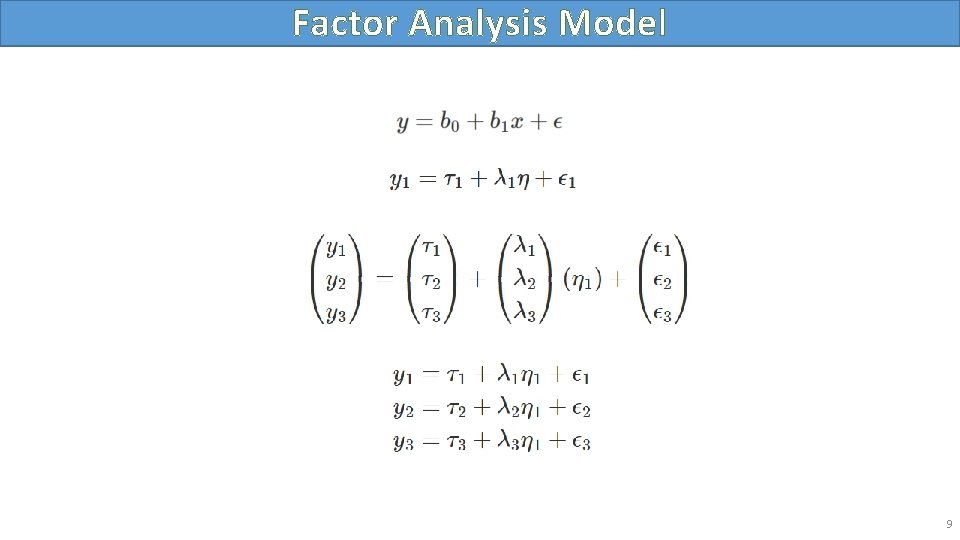
Factor Analysis Model 9

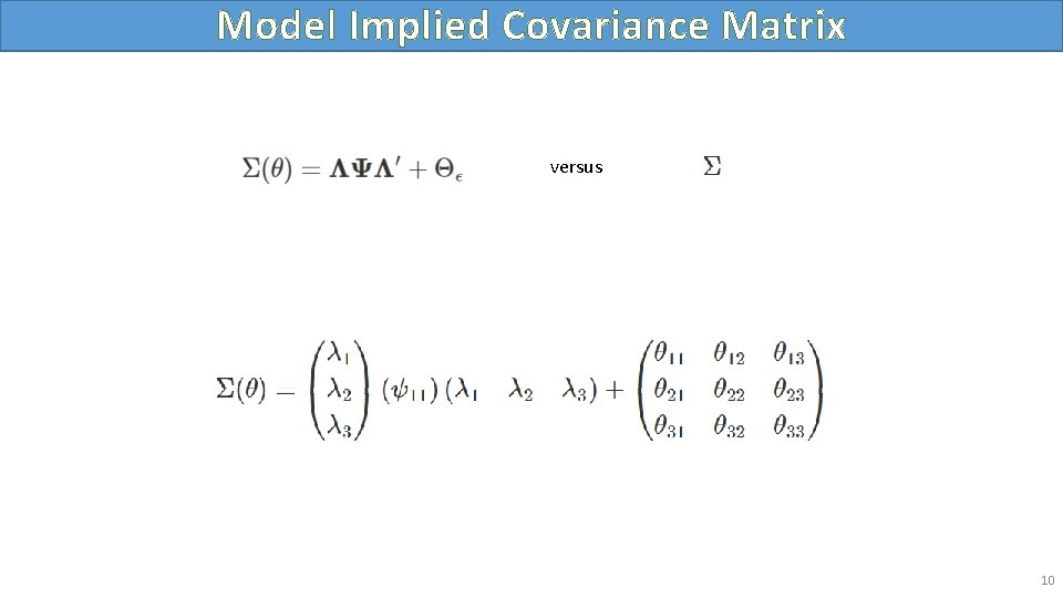
Model Implied Covariance Matrix versus 10

Path Diagram 11

Measurement vs. Covariance Model 12

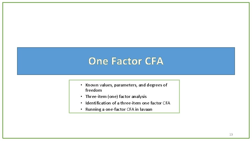
One Factor CFA • Known values, parameters, and degrees of freedom • Three-item (one) factor analysis • Identification of a three-item one factor CFA • Running a one-factor CFA in lavaan 13

One Factor CFA 14

Sample Covariance Matrix versus > round(cov(dat[, 3: 5]), 2) q 03 q 04 q 05 q 03 1. 16 -0. 39 -0. 32 q 04 -0. 39 0. 90 0. 37 q 05 -0. 32 0. 37 0. 90 15

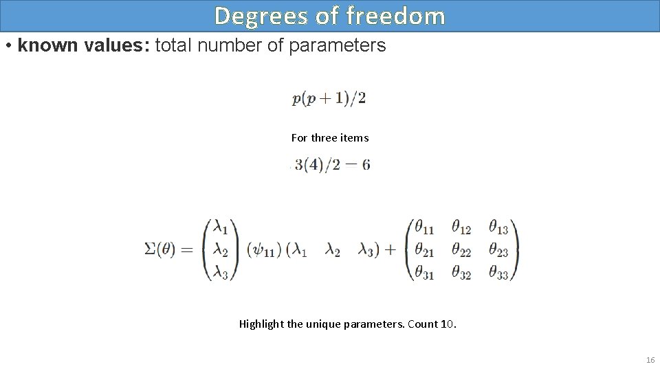
Degrees of freedom • known values: total number of parameters For three items Highlight the unique parameters. Count 10. 16

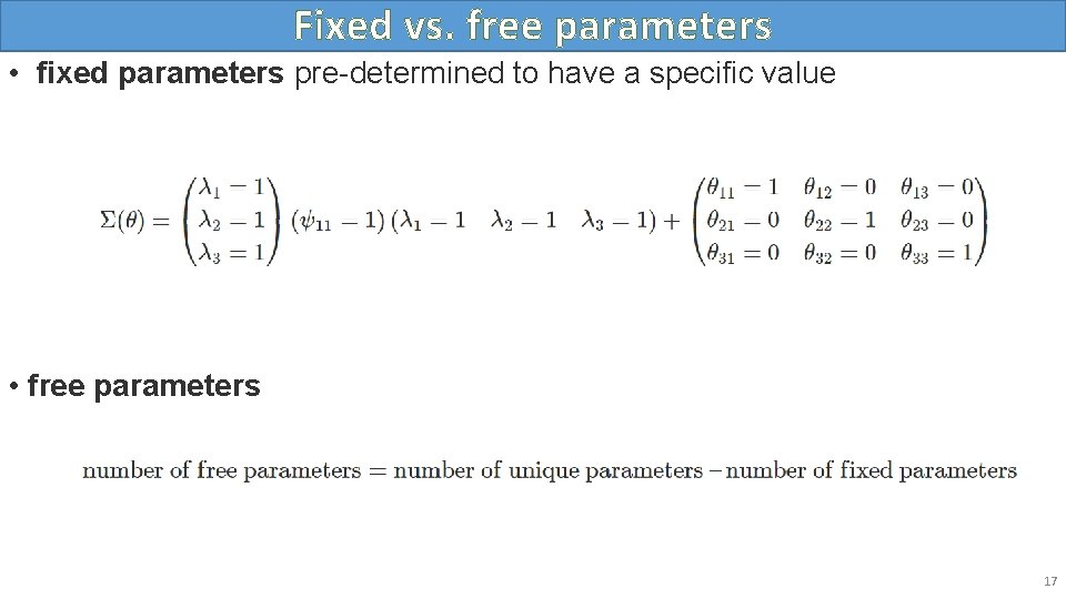
Fixed vs. free parameters • fixed parameters pre-determined to have a specific value • free parameters 17

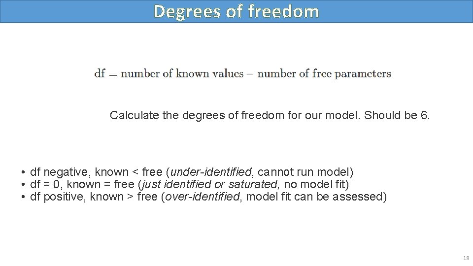
Degrees of freedom Calculate the degrees of freedom for our model. Should be 6. • df negative, known < free (under-identified, cannot run model) • df = 0, known = free (just identified or saturated, no model fit) • df positive, known > free (over-identified, model fit can be assessed) 18

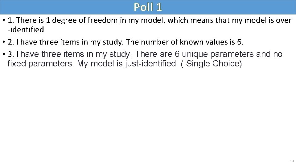
Poll 1 • 1. There is 1 degree of freedom in my model, which means that my model is over -identified • 2. I have three items in my study. The number of known values is 6. • 3. I have three items in my study. There are 6 unique parameters and no fixed parameters. My model is just-identified. ( Single Choice) 19

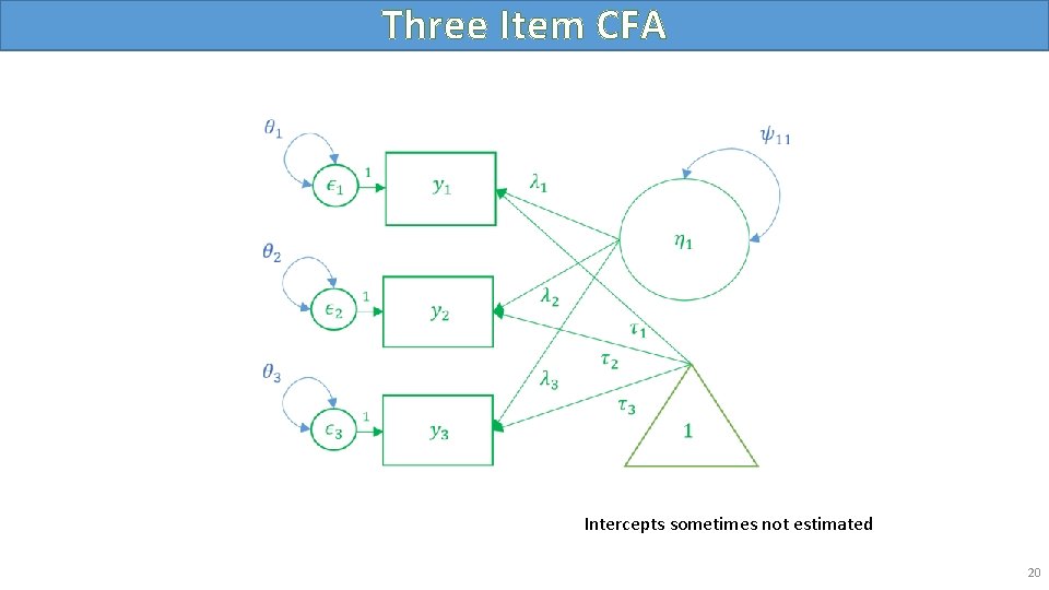
Three Item CFA Intercepts sometimes not estimated 20

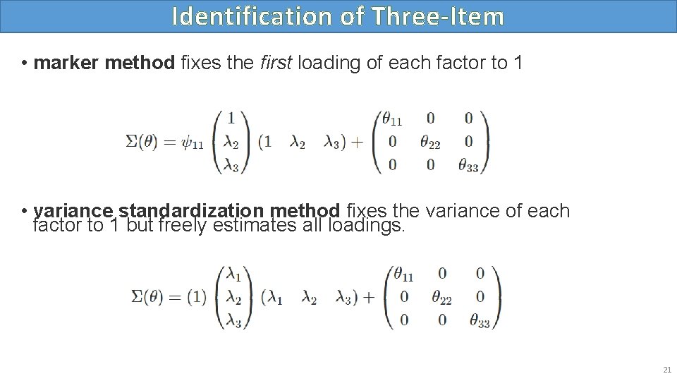
Identification of Three-Item • marker method fixes the first loading of each factor to 1 • variance standardization method fixes the variance of each factor to 1 but freely estimates all loadings. 21

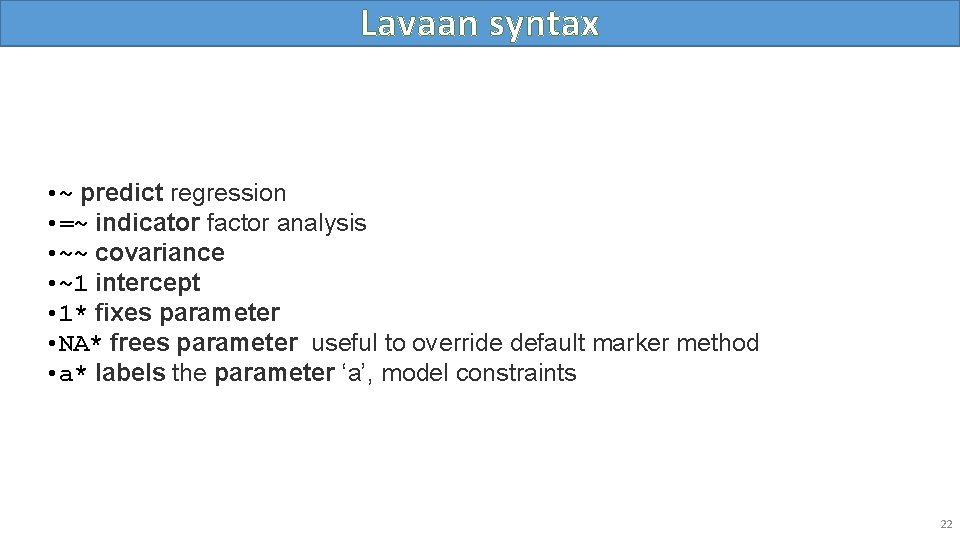
Lavaan syntax • ~ predict regression • =~ indicator factor analysis • ~~ covariance • ~1 intercept • 1* fixes parameter • NA* frees parameter useful to override default marker method • a* labels the parameter ‘a’, model constraints 22

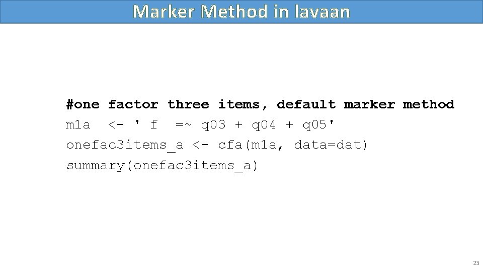
Marker Method in lavaan #one factor three items, default marker method m 1 a <- ' f =~ q 03 + q 04 + q 05' onefac 3 items_a <- cfa(m 1 a, data=dat) summary(onefac 3 items_a) 23

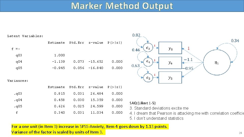
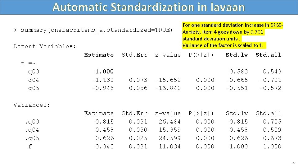
Marker Method Output Latent Variables: Estimate Std. Err z-value P(>|z|) f =~ q 03 1. 000 q 04 -1. 139 0. 073 -15. 652 0. 000 q 05 -0. 945 0. 056 -16. 840 0. 000 Estimate Std. Err z-value P(>|z|) . q 03 0. 815 0. 031 26. 484 0. 000 . q 04 0. 458 0. 030 15. 359 0. 000 . q 05 0. 626 0. 025 24. 599 0. 000 0. 340 0. 031 11. 034 0. 000 Variances: f SAQ (Likert 1 -5) 3. Standard deviations excite me 4. I dream that Pearson is attacking me with correlation coefficie 5. I don’t understand statistics For a one unit (in Item 3) increase in SPSS-Anxiety, Item 4 goes down by 1. 13 points. Variance of the factor is scaled by units of Item 3. 24

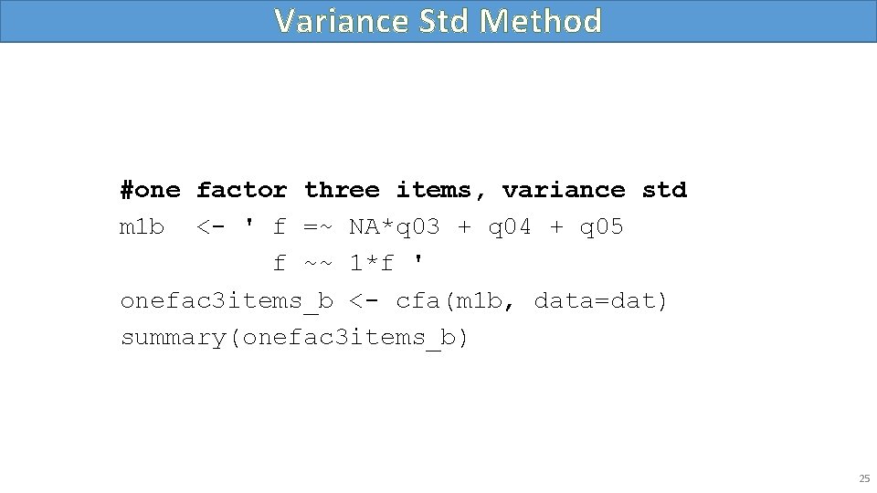
Variance Std Method #one factor three items, variance std m 1 b <- ' f =~ NA*q 03 + q 04 + q 05 f ~~ 1*f ' onefac 3 items_b <- cfa(m 1 b, data=dat) summary(onefac 3 items_b) 25

Variance Std Output Latent Variables: Estimate Std. Err z-value P(>|z|) q 03 0. 583 0. 026 22. 067 0. 000 q 04 -0. 665 0. 026 -25. 605 0. 000 q 05 -0. 551 0. 024 -22. 800 0. 000 Estimate Std. Err z-value P(>|z|) f =~ Variances: f 1. 000 . q 03 0. 815 0. 031 26. 484 0. 000 . q 04 0. 458 0. 030 15. 359 0. 000 . q 05 0. 626 0. 025 24. 599 0. 000 SAQ (Likert 1 -5) 3. Standard deviations excite me 4. I dream that Pearson is attacking me with correlation coefficie 5. I don’t understand statistics For one standard deviation increase in SPSS-Anxiety, Item 4 goes down by 0. 665 points. Variance of the factor is scaled to 1. 26

Automatic Standardization in lavaan > summary(onefac 3 items_a, standardized=TRUE) Latent Variables: Estimate f =~ q 03 q 04 q 05 Std. Err z-value For one standard deviation increase in SPSSAnxiety, Item 4 goes down by 0. 701 standard deviation units. Variance of the factor is scaled to 1. P(>|z|) Std. lv Std. all 0. 543 -0. 701 -0. 572 Std. all 0. 705 0. 509 0. 673 1. 000 -1. 139 -0. 945 0. 073 0. 056 -15. 652 -16. 840 0. 000 0. 583 -0. 665 -0. 551 Estimate 0. 815 0. 458 0. 626 0. 340 Std. Err 0. 031 0. 030 0. 025 0. 031 z-value 26. 484 15. 359 24. 599 11. 034 P(>|z|) 0. 000 Std. lv 0. 815 0. 458 0. 626 1. 000 Variances: . q 03. q 04. q 05 f 27

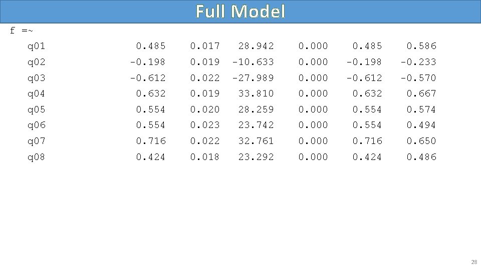
Full Model f =~ q 01 0. 485 0. 017 28. 942 0. 000 0. 485 0. 586 q 02 -0. 198 0. 019 -10. 633 0. 000 -0. 198 -0. 233 q 03 -0. 612 0. 022 -27. 989 0. 000 -0. 612 -0. 570 q 04 0. 632 0. 019 33. 810 0. 000 0. 632 0. 667 q 05 0. 554 0. 020 28. 259 0. 000 0. 554 0. 574 q 06 0. 554 0. 023 23. 742 0. 000 0. 554 0. 494 q 07 0. 716 0. 022 32. 761 0. 000 0. 716 0. 650 q 08 0. 424 0. 018 23. 292 0. 000 0. 424 0. 486 28

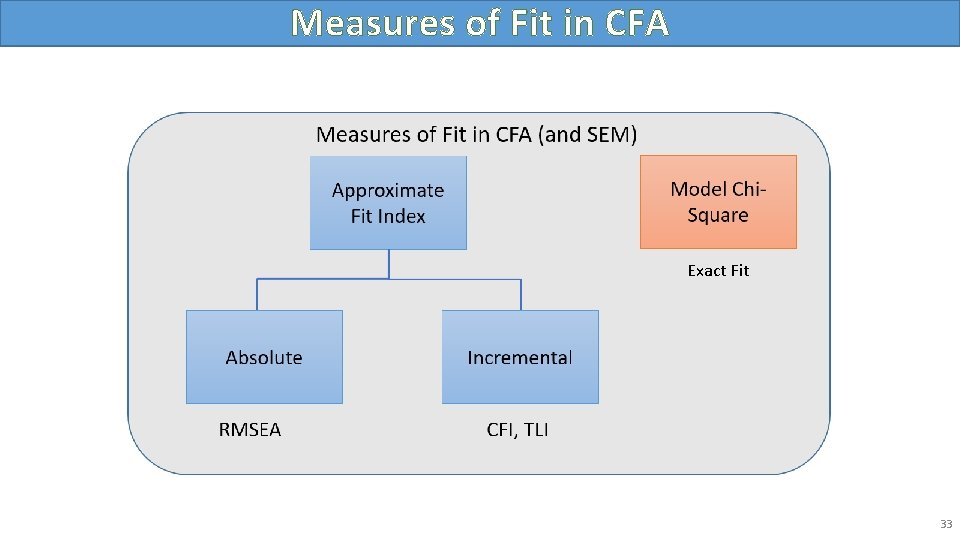
Model Fit Statistics • Model chi-square • Approximate fit indices • CFI / TLI / RMSEA 29

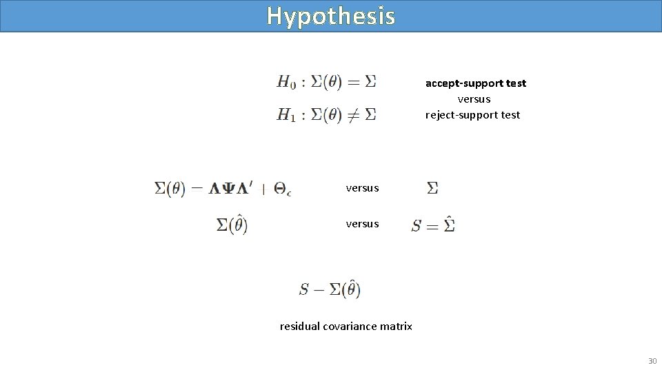
Hypothesis accept-support test versus reject-support test versus residual covariance matrix 30

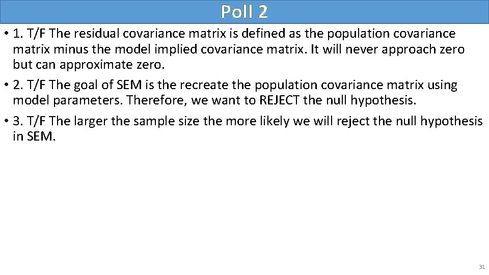
Poll 2 • 1. T/F The residual covariance matrix is defined as the population covariance matrix minus the model implied covariance matrix. It will never approach zero but can approximate zero. • 2. T/F The goal of SEM is the recreate the population covariance matrix using model parameters. Therefore, we want to REJECT the null hypothesis. • 3. T/F The larger the sample size the more likely we will reject the null hypothesis in SEM. 31

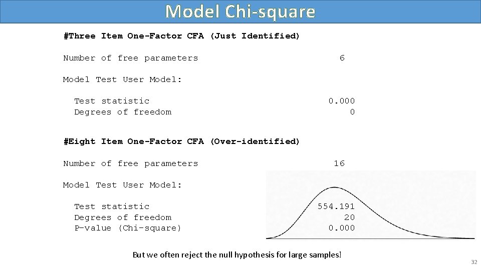
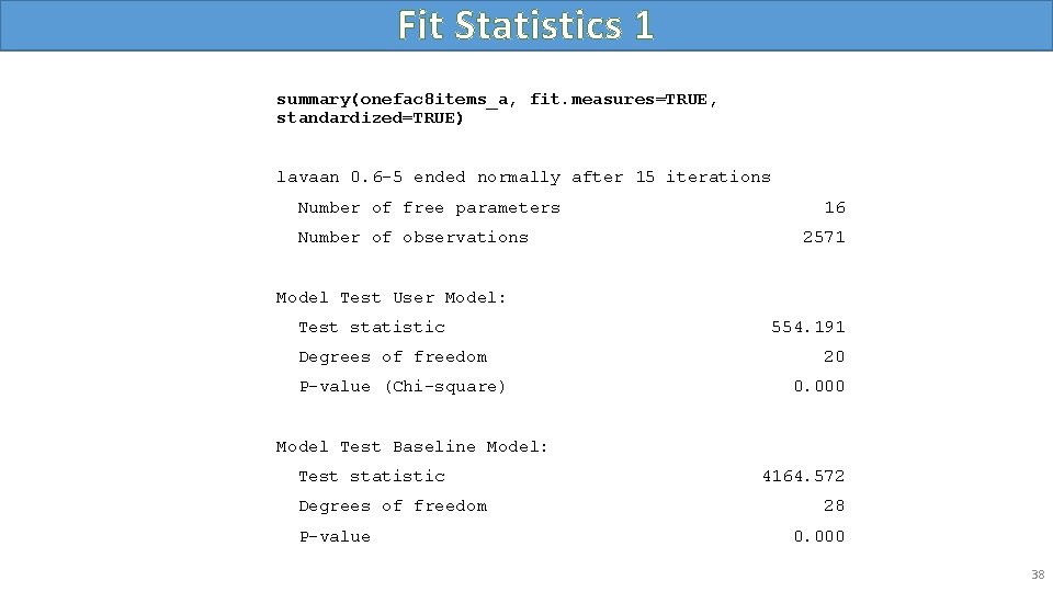
Model Chi-square #Three Item One-Factor CFA (Just Identified) Number of free parameters 6 Model Test User Model: Test statistic Degrees of freedom 0. 000 0 #Eight Item One-Factor CFA (Over-identified) Number of free parameters 16 Model Test User Model: Test statistic Degrees of freedom P-value (Chi-square) 554. 191 20 0. 000 But we often reject the null hypothesis for large samples! 32

Measures of Fit in CFA Exact Fit 33

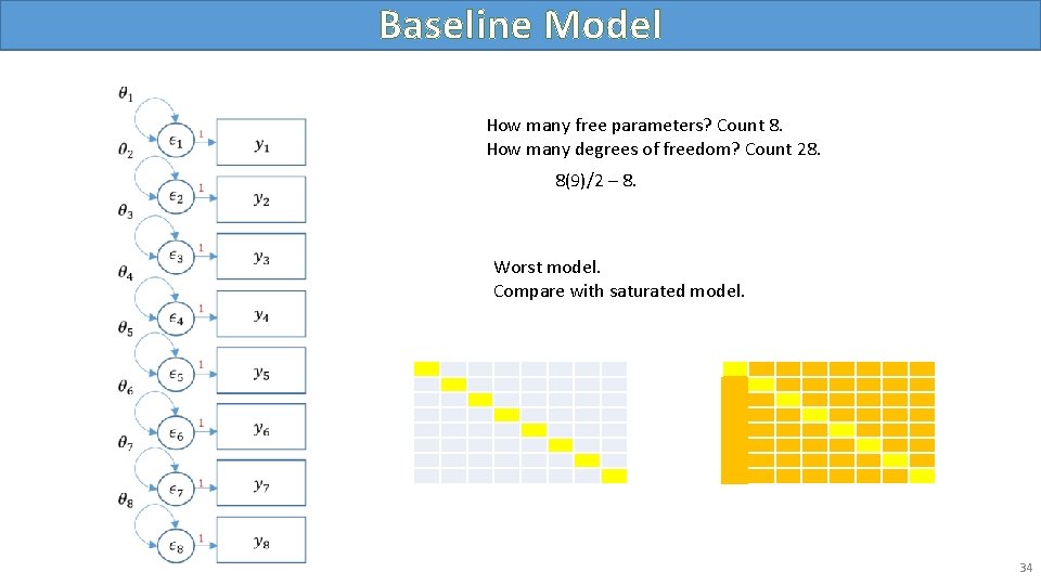
Baseline Model How many free parameters? Count 8. How many degrees of freedom? Count 28. 8(9)/2 – 8. Worst model. Compare with saturated model. 34

Baseline 35

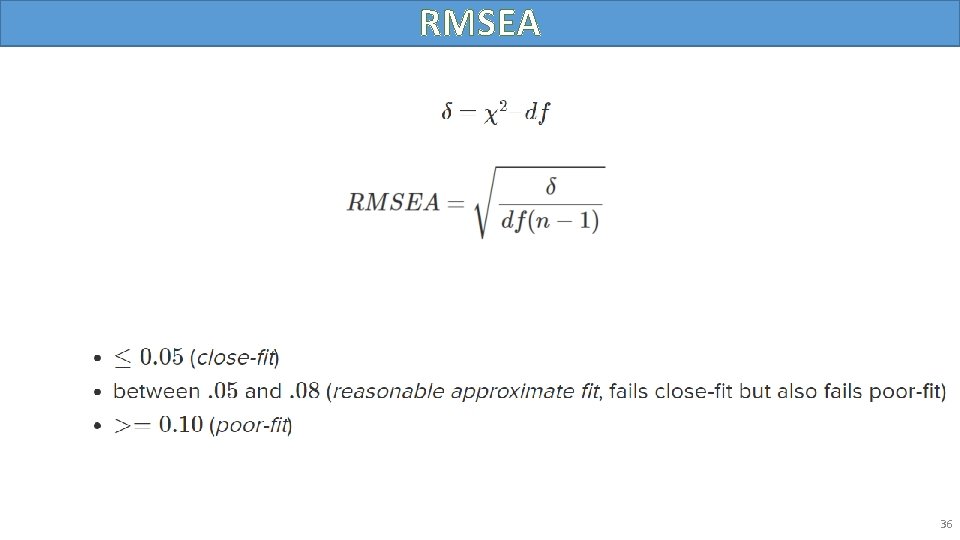
RMSEA 36

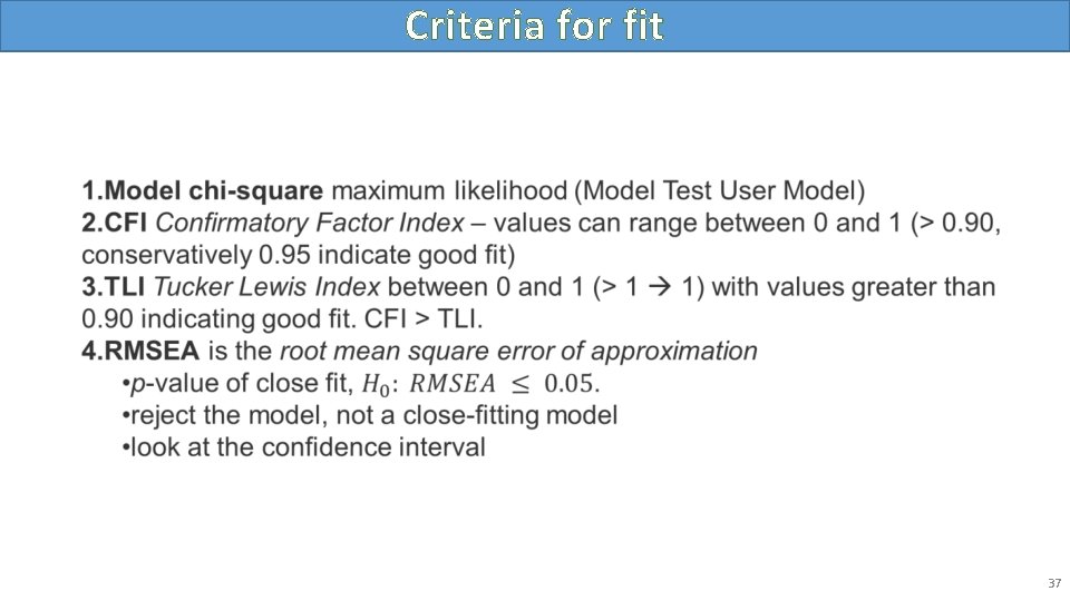
Criteria for fit • 37

Fit Statistics 1 summary(onefac 8 items_a, fit. measures=TRUE, standardized=TRUE) lavaan 0. 6 -5 ended normally after 15 iterations Number of free parameters Number of observations 16 2571 Model Test User Model: Test statistic Degrees of freedom P-value (Chi-square) 554. 191 20 0. 000 Model Test Baseline Model: Test statistic Degrees of freedom P-value 4164. 572 28 0. 000 38

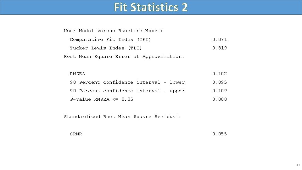
Fit Statistics 2 User Model versus Baseline Model: Comparative Fit Index (CFI) 0. 871 Tucker-Lewis Index (TLI) 0. 819 Root Mean Square Error of Approximation: RMSEA 0. 102 90 Percent confidence interval - lower 0. 095 90 Percent confidence interval - upper 0. 109 P-value RMSEA <= 0. 05 0. 000 Standardized Root Mean Square Residual: SRMR 0. 055 39

Two Factor Confirmatory Factor Analysis • Correlated factors • Uncorrelated factors 40

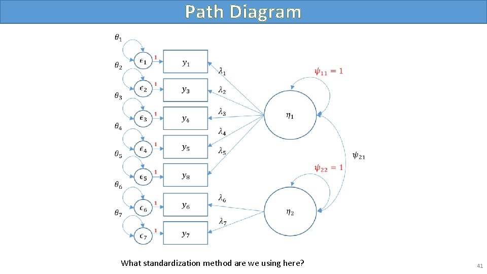
Path Diagram What standardization method are we using here? 41

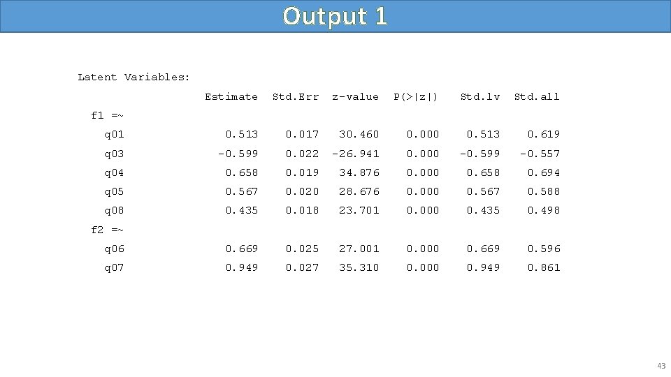
Correlated Factors #correlated two factor solution, marker method m 4 b <- 'f 1 =~ q 01+ q 03 + q 04 + q 05 + q 08 f 2 =~ q 06 + q 07' twofac 7 items_b <- cfa(m 4 b, data=dat, std. lv=TRUE) summary(twofac 7 items_b, fit. measures=TRUE, standardized=TRUE) 42

Output 1 Latent Variables: Estimate Std. Err z-value P(>|z|) Std. lv Std. all q 01 0. 513 0. 017 30. 460 0. 000 0. 513 0. 619 q 03 -0. 599 0. 022 -26. 941 0. 000 -0. 599 -0. 557 q 04 0. 658 0. 019 34. 876 0. 000 0. 658 0. 694 q 05 0. 567 0. 020 28. 676 0. 000 0. 567 0. 588 q 08 0. 435 0. 018 23. 701 0. 000 0. 435 0. 498 q 06 0. 669 0. 025 27. 001 0. 000 0. 669 0. 596 q 07 0. 949 0. 027 35. 310 0. 000 0. 949 0. 861 f 1 =~ f 2 =~ 43

Output 2 Covariances: Estimate Std. Err z-value P(>|z|) Std. lv Std. all 0. 676 0. 020 33. 023 0. 000 0. 676 Estimate Std. Err z-value P(>|z|) Std. lv Std. all . q 01 0. 423 0. 014 29. 157 0. 000 0. 423 0. 617 . q 03 0. 796 0. 026 31. 025 0. 000 0. 796 0. 689 . q 04 0. 466 0. 018 25. 824 0. 000 0. 466 0. 518 . q 05 0. 608 0. 020 30. 173 0. 000 0. 608 0. 654 . q 08 0. 572 0. 018 32. 332 0. 000 0. 572 0. 752 . q 06 0. 811 0. 030 27. 187 0. 000 0. 811 0. 644 . q 07 0. 314 0. 040 7. 815 0. 000 0. 314 0. 258 f 1 1. 000 f 2 1. 000 f 1 ~~ f 2 Variances: 44

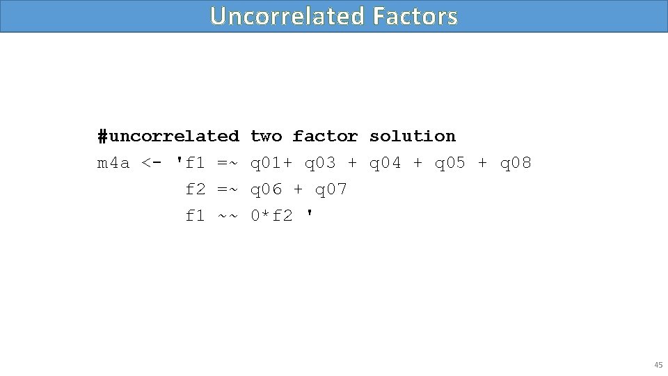
Uncorrelated Factors #uncorrelated m 4 a <- 'f 1 =~ f 2 =~ f 1 ~~ two factor solution q 01+ q 03 + q 04 + q 05 + q 08 q 06 + q 07 0*f 2 ' 45

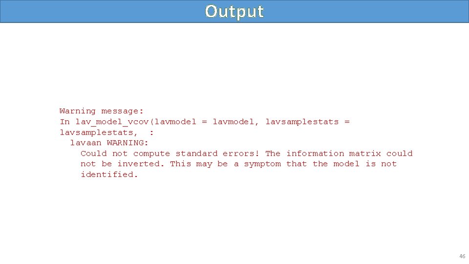
Output Warning message: In lav_model_vcov(lavmodel = lavmodel, lavsamplestats = lavsamplestats, : lavaan WARNING: Could not compute standard errors! The information matrix could not be inverted. This may be a symptom that the model is not identified. 46

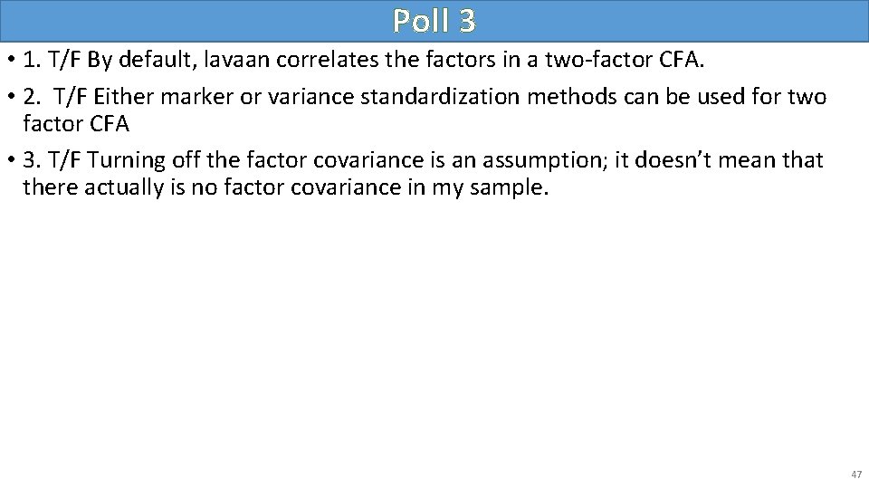
Poll 3 • 1. T/F By default, lavaan correlates the factors in a two-factor CFA. • 2. T/F Either marker or variance standardization methods can be used for two factor CFA • 3. T/F Turning off the factor covariance is an assumption; it doesn’t mean that there actually is no factor covariance in my sample. 47

Intermission • This concludes the lecture portion of the seminar. • We will go over three exercises in the following section. 48

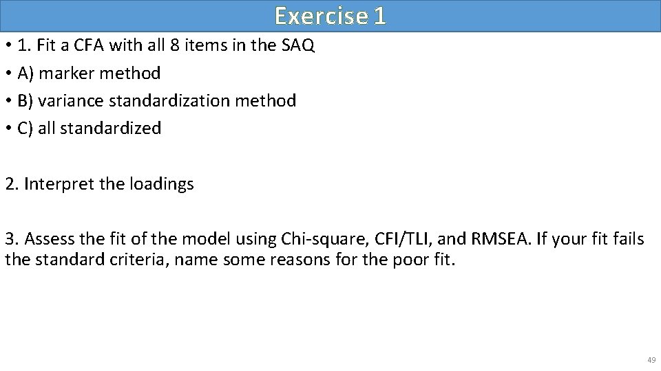
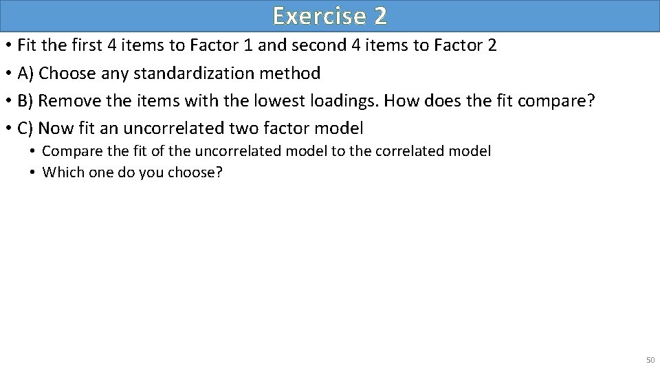
Exercise 1 • 1. Fit a CFA with all 8 items in the SAQ • A) marker method • B) variance standardization method • C) all standardized 2. Interpret the loadings 3. Assess the fit of the model using Chi-square, CFI/TLI, and RMSEA. If your fit fails the standard criteria, name some reasons for the poor fit. 49

Exercise 2 • Fit the first 4 items to Factor 1 and second 4 items to Factor 2 • A) Choose any standardization method • B) Remove the items with the lowest loadings. How does the fit compare? • C) Now fit an uncorrelated two factor model • Compare the fit of the uncorrelated model to the correlated model • Which one do you choose? 50

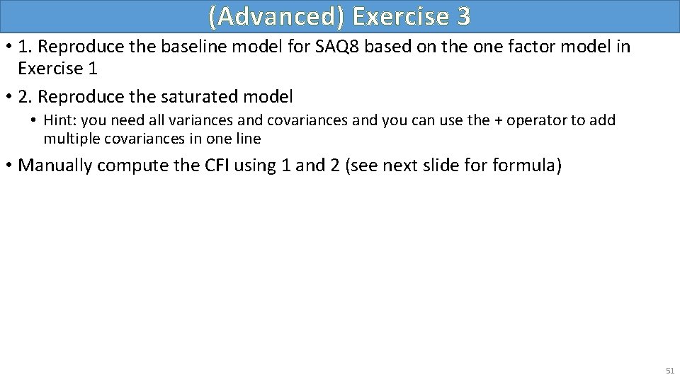
(Advanced) Exercise 3 • 1. Reproduce the baseline model for SAQ 8 based on the one factor model in Exercise 1 • 2. Reproduce the saturated model • Hint: you need all variances and covariances and you can use the + operator to add multiple covariances in one line • Manually compute the CFI using 1 and 2 (see next slide formula) 51

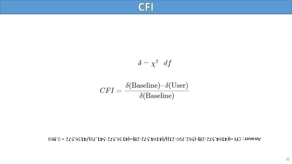
52 Answer: CFI =((4164. 572 -28)-(562. 790 -21))/(4164. 572 -28)=(4136. 572 -541. 79)/4136. 572 = 0. 869 CFI

More Advanced Topics • Two-item factor analysis • Uncorrelated factor analysis with two items • Second order factors 53

Thank you! Any questions? 54