CONFIDENCE INTERVALS probability density function of b 2

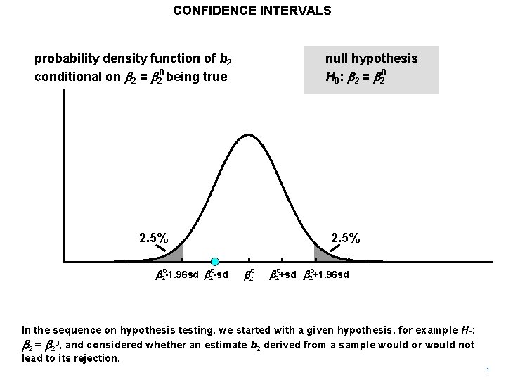
CONFIDENCE INTERVALS probability density function of b 2 conditional on b 2 = b 20 being true null hypothesis H 0: b 2 = b 20 2. 5% b 20 -1. 96 sd b 20 -sd 2. 5% b 20+sd b 20+1. 96 sd In the sequence on hypothesis testing, we started with a given hypothesis, for example H 0: b 2 = b 20, and considered whether an estimate b 2 derived from a sample would or would not lead to its rejection. 1

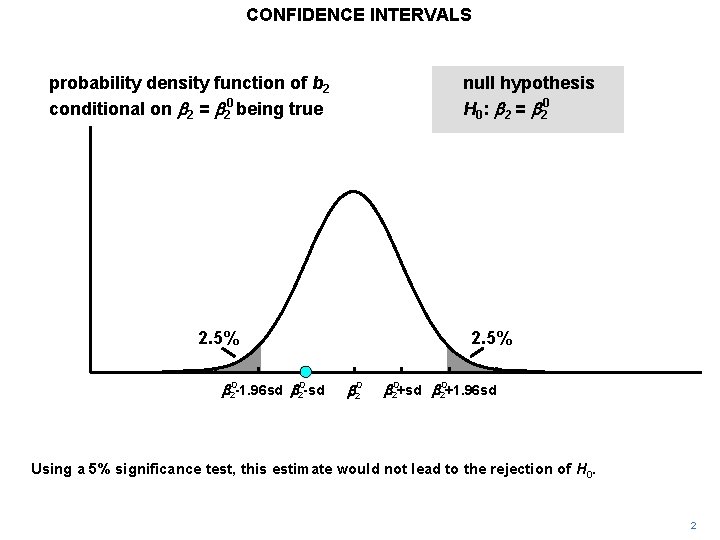
CONFIDENCE INTERVALS probability density function of b 2 conditional on b 2 = b 20 being true null hypothesis H 0: b 2 = b 20 2. 5% b 20 -1. 96 sd b 20 -sd 2. 5% b 20+sd b 20+1. 96 sd Using a 5% significance test, this estimate would not lead to the rejection of H 0. 2

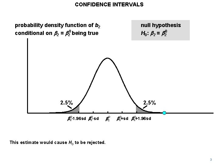
CONFIDENCE INTERVALS probability density function of b 2 conditional on b 2 = b 20 being true null hypothesis H 0: b 2 = b 20 2. 5% b 20 -1. 96 sd b 20 -sd 2. 5% b 20+sd b 20+1. 96 sd This estimate would cause H 0 to be rejected. 3

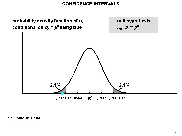
CONFIDENCE INTERVALS probability density function of b 2 conditional on b 2 = b 20 being true null hypothesis H 0: b 2 = b 20 2. 5% b 20 -1. 96 sd b 20 -sd 2. 5% b 20+sd b 20+1. 96 sd So would this one. 4

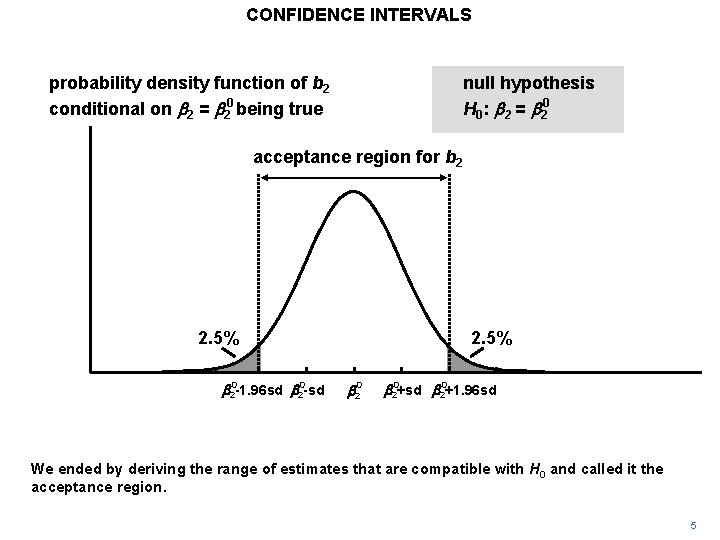
CONFIDENCE INTERVALS probability density function of b 2 conditional on b 2 = b 20 being true null hypothesis H 0: b 2 = b 20 acceptance region for b 2 2. 5% b 20 -1. 96 sd b 20 -sd 2. 5% b 20+sd b 20+1. 96 sd We ended by deriving the range of estimates that are compatible with H 0 and called it the acceptance region. 5

CONFIDENCE INTERVALS b 2 Now we will do exactly the opposite. Given a sample estimate, we will find the set of hypotheses that would not be contradicted by it, using a two-tailed 5% significance test. 6

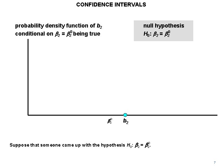
CONFIDENCE INTERVALS probability density function of b 2 conditional on b 2 = b 20 being true null hypothesis H 0: b 2 = b 20 b 2 Suppose that someone came up with the hypothesis H 0: b 2 = b 2. 0 7

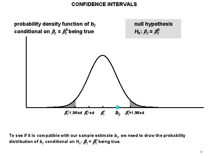
CONFIDENCE INTERVALS probability density function of b 2 conditional on b 2 = b 20 being true b 20 -1. 96 sd b 20 -sd null hypothesis H 0: b 2 = b 20+1. 96 sd To see if it is compatible with our sample estimate b 2, we need to draw the probability distribution of b 2 conditional on H 0: b 2 = b 20 being true. 8

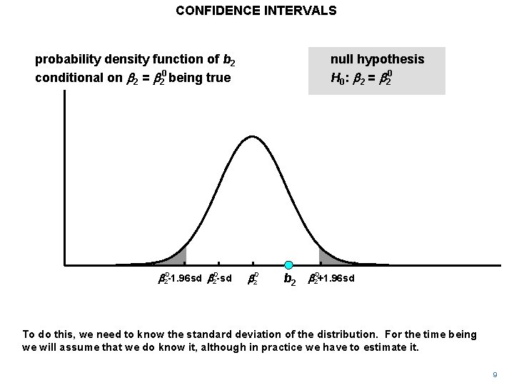
CONFIDENCE INTERVALS probability density function of b 2 conditional on b 2 = b 20 being true b 20 -1. 96 sd b 20 -sd null hypothesis H 0: b 2 = b 20+1. 96 sd To do this, we need to know the standard deviation of the distribution. For the time being we will assume that we do know it, although in practice we have to estimate it. 9

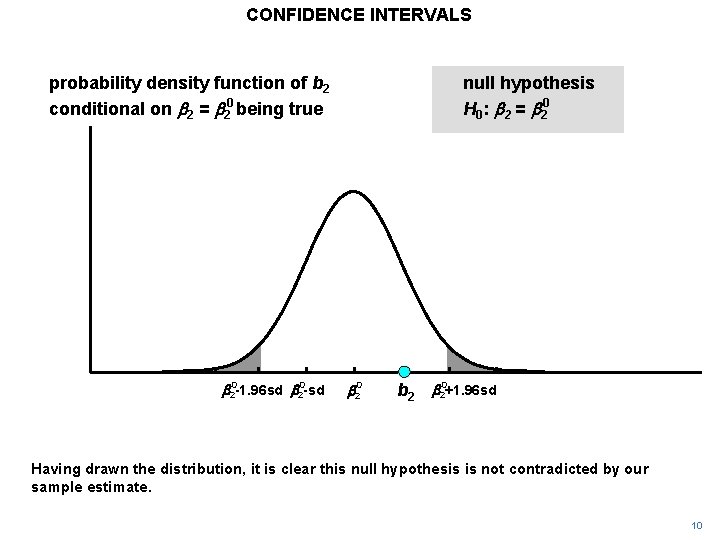
CONFIDENCE INTERVALS probability density function of b 2 conditional on b 2 = b 20 being true b 20 -1. 96 sd b 20 -sd null hypothesis H 0: b 2 = b 20+1. 96 sd Having drawn the distribution, it is clear this null hypothesis is not contradicted by our sample estimate. 10

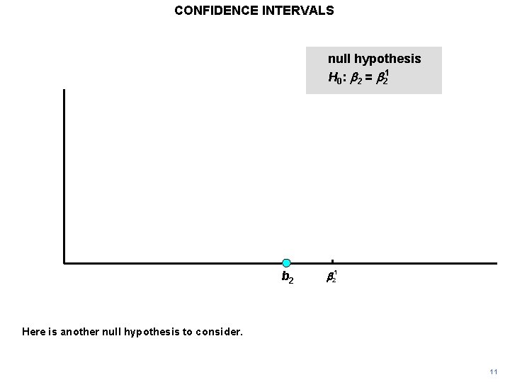
CONFIDENCE INTERVALS null hypothesis H 0: b 2 = b 21 Here is another null hypothesis to consider. 11

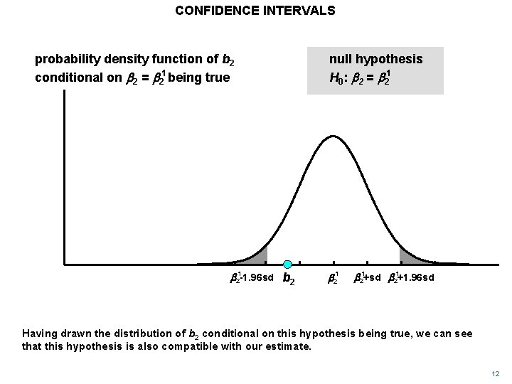
CONFIDENCE INTERVALS probability density function of b 2 conditional on b 2 = b 21 being true b 21 -1. 96 sd null hypothesis H 0: b 2 = b 21+sd b 21+1. 96 sd Having drawn the distribution of b 2 conditional on this hypothesis being true, we can see that this hypothesis is also compatible with our estimate. 12

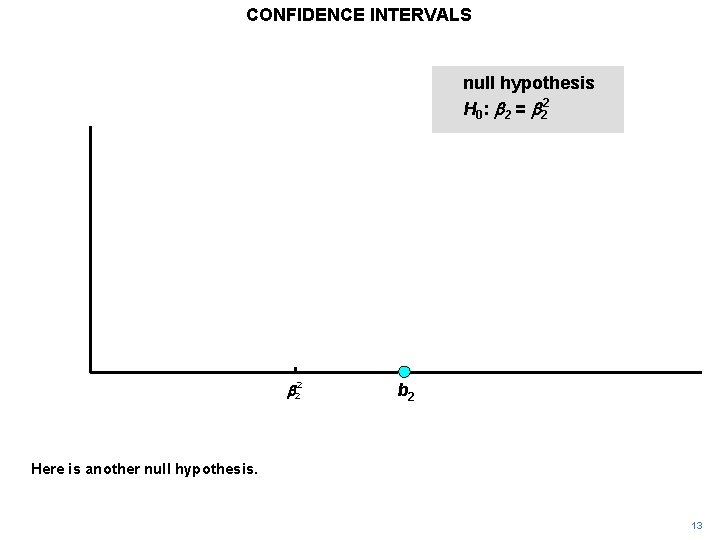
CONFIDENCE INTERVALS null hypothesis H 0: b 2 = b 22 b 2 Here is another null hypothesis. 13

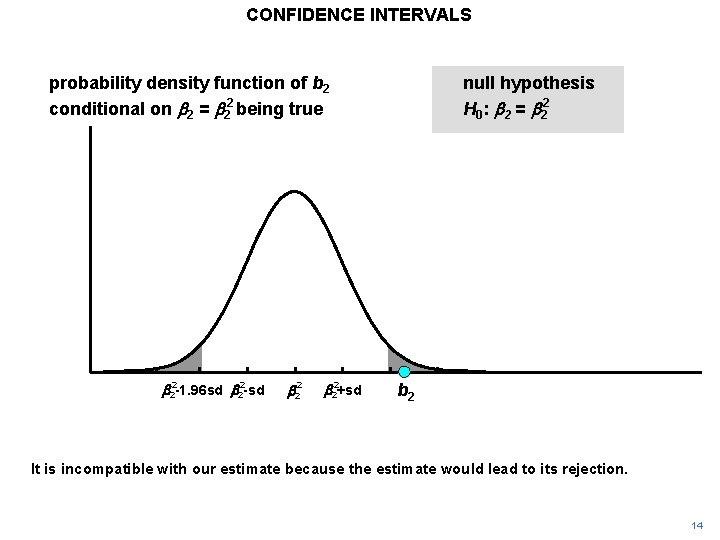
CONFIDENCE INTERVALS probability density function of b 2 conditional on b 2 = b 22 being true b 22 -1. 96 sd b 22 -sd b 22+sd null hypothesis H 0: b 2 = b 22 b 2 It is incompatible with our estimate because the estimate would lead to its rejection. 14

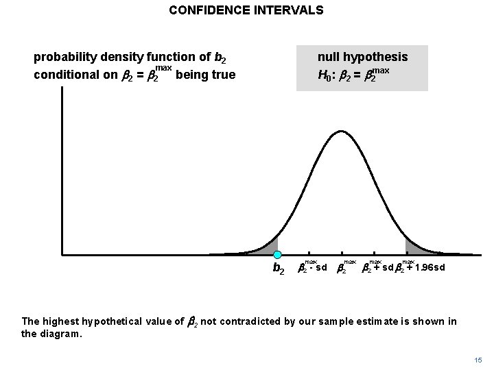
CONFIDENCE INTERVALS probability density function of b 2 max conditional on b 2 = b 2 being true null hypothesis H 0: b 2 = b 2 max b 2 - sd max b 2 + sd b 2 + 1. 96 sd The highest hypothetical value of b 2 not contradicted by our sample estimate is shown in the diagram. 15

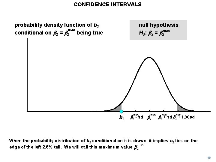
CONFIDENCE INTERVALS probability density function of b 2 max conditional on b 2 = b 2 being true null hypothesis H 0: b 2 = b 2 max b 2 - sd max b 2 + sd b 2 + 1. 96 sd When the probability distribution of b 2 conditional on it is drawn, it implies b 2 lies on the max edge of the left 2. 5% tail. We will call this maximum value b 2. 16

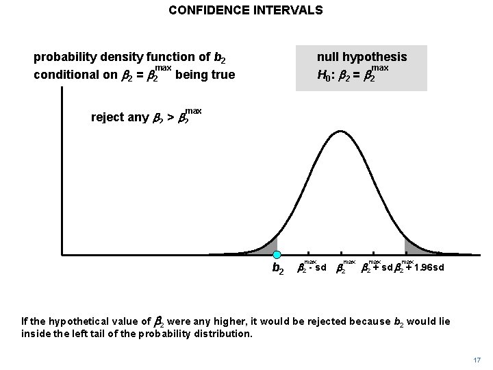
CONFIDENCE INTERVALS probability density function of b 2 max conditional on b 2 = b 2 being true null hypothesis max H 0 : b 2 = b 2 max reject any b 2 > b 2 max b 2 = b 2 max b 2 - 1. 96 sd = b 2 + 1. 96 sd reject any b 2 > b 2 + 1. 96 sd b 2 max b 2 - sd max b 2 + sd b 2 + 1. 96 sd If the hypothetical value of b 2 were any higher, it would be rejected because b 2 would lie inside the left tail of the probability distribution. 17

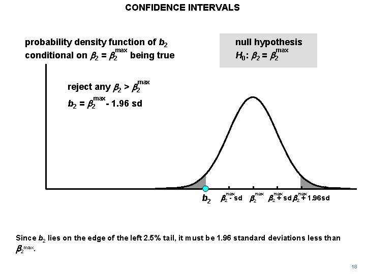
CONFIDENCE INTERVALS probability density function of b 2 max conditional on b 2 = b 2 being true null hypothesis max H 0 : b 2 = b 2 max reject any b 2 > b 2 max b 2 = b 2 max b 2 - 1. 96 sd = b 2 + 1. 96 sd reject any b 2 > b 2 + 1. 96 sd b 2 max b 2 - sd max b 2 + sd b 2 + 1. 96 sd Since b 2 lies on the edge of the left 2. 5% tail, it must be 1. 96 standard deviations less than b 2 max. 18

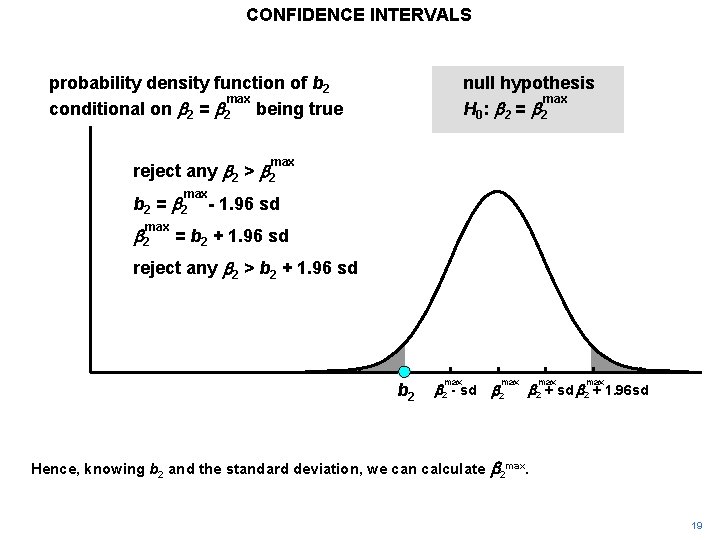
CONFIDENCE INTERVALS probability density function of b 2 max conditional on b 2 = b 2 being true null hypothesis max H 0 : b 2 = b 2 max reject any b 2 > b 2 max b 2 = b 2 max b 2 - 1. 96 sd = b 2 + 1. 96 sd reject any b 2 > b 2 + 1. 96 sd b 2 max b 2 - sd Hence, knowing b 2 and the standard deviation, we can calculate max b 2 + sd b 2 + 1. 96 sd b 2 max. 19

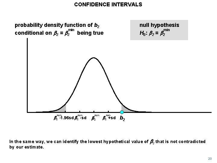
CONFIDENCE INTERVALS probability density function of b 2 min conditional on b 2 = b 2 being true min b 2 -1. 96 sd b 2 -sd min b 2 null hypothesis min H 0 : b 2 = b 2 min b 2 +sd b 2 In the same way, we can identify the lowest hypothetical value of by our estimate. b 2 that is not contradicted 20

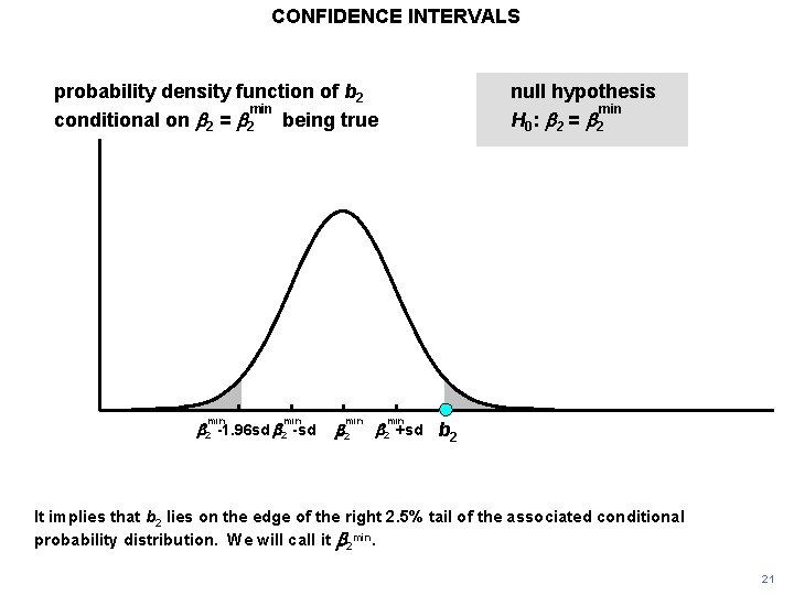
CONFIDENCE INTERVALS probability density function of b 2 min conditional on b 2 = b 2 being true min b 2 -1. 96 sd b 2 -sd min b 2 null hypothesis min H 0 : b 2 = b 2 min b 2 +sd b 2 It implies that b 2 lies on the edge of the right 2. 5% tail of the associated conditional probability distribution. We will call it b 2 min. 21

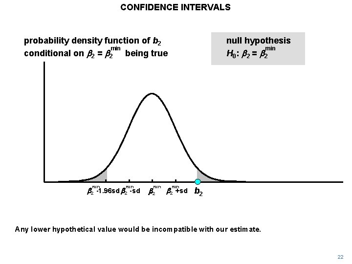
CONFIDENCE INTERVALS probability density function of b 2 min conditional on b 2 = b 2 being true min b 2 -1. 96 sd b 2 -sd min b 2 null hypothesis min H 0 : b 2 = b 2 min b 2 +sd b 2 Any lower hypothetical value would be incompatible with our estimate. 22

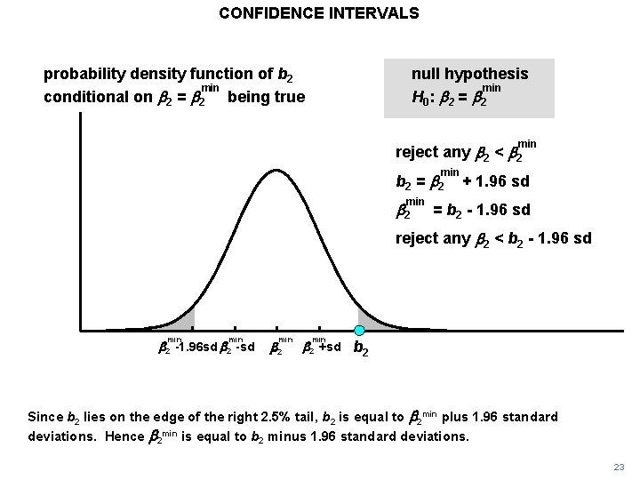
CONFIDENCE INTERVALS probability density function of b 2 min conditional on b 2 = b 2 being true null hypothesis min H 0 : b 2 = b 2 min reject any b 2 < b 2 min b 2 = b 2 min b 2 + 1. 96 sd = b 2 - 1. 96 sd reject any b 2 < b 2 - 1. 96 sd min b 2 -1. 96 sd b 2 -sd min b 2 +sd b 2 Since b 2 lies on the edge of the right 2. 5% tail, b 2 is equal to b 2 min plus 1. 96 standard deviations. Hence b 2 min is equal to b 2 minus 1. 96 standard deviations. 23

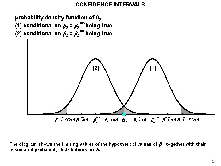
CONFIDENCE INTERVALS probability density function of b 2 max (1) conditional on b 2 = b 2 being true min (2) conditional on b 2 = b 2 being true (2) min b 2 -1. 96 sd b 2 -sd min b 2 (1) min b 2 +sd b 2 max b 2 - sd max b 2 The diagram shows the limiting values of the hypothetical values of associated probability distributions for b 2. max b 2 + sd b 2 + 1. 96 sd b 2, together with their 24

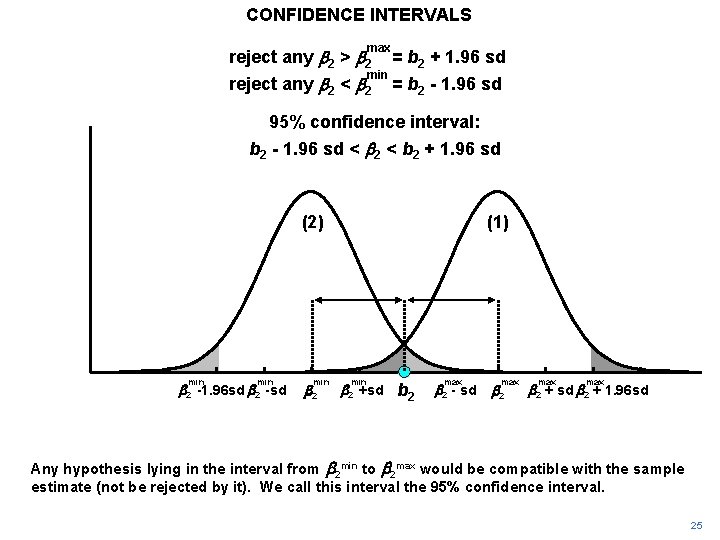
CONFIDENCE INTERVALS max reject any b 2 > b 2 = b 2 + 1. 96 sd reject any b 2 < b 2 = b 2 - 1. 96 sd min 95% confidence interval: b 2 - 1. 96 sd < b 2 + 1. 96 sd (2) min b 2 -1. 96 sd b 2 -sd min b 2 (1) min b 2 +sd b 2 max b 2 - sd max b 2 + sd b 2 + 1. 96 sd Any hypothesis lying in the interval from b 2 min to b 2 max would be compatible with the sample estimate (not be rejected by it). We call this interval the 95% confidence interval. 25

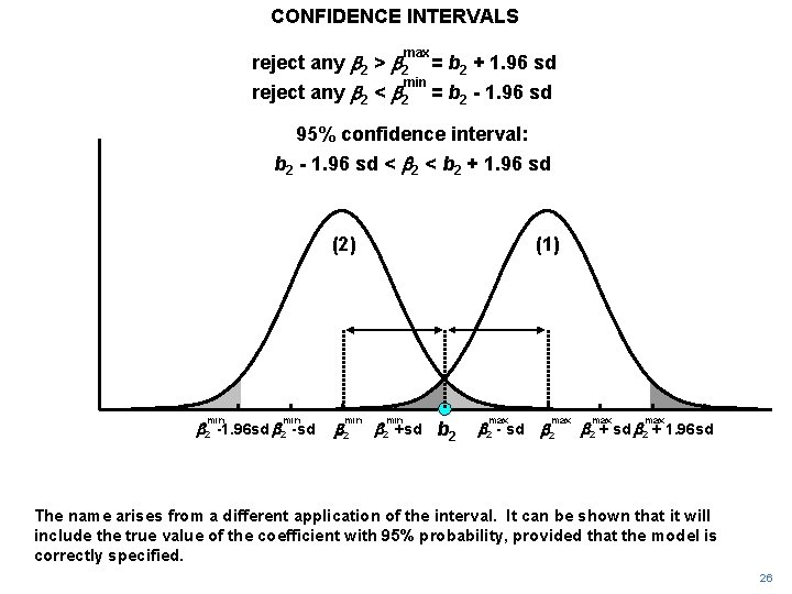
CONFIDENCE INTERVALS max reject any b 2 > b 2 = b 2 + 1. 96 sd reject any b 2 < b 2 = b 2 - 1. 96 sd min 95% confidence interval: b 2 - 1. 96 sd < b 2 + 1. 96 sd (2) min b 2 -1. 96 sd b 2 -sd min b 2 (1) min b 2 +sd b 2 max b 2 - sd max b 2 + sd b 2 + 1. 96 sd The name arises from a different application of the interval. It can be shown that it will include the true value of the coefficient with 95% probability, provided that the model is correctly specified. 26

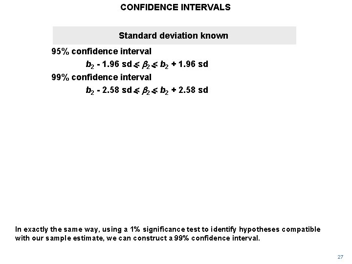
CONFIDENCE INTERVALS Standard deviation known 95% confidence interval b 2 - 1. 96 sd < b 2 + 1. 96 sd 99% confidence interval b 2 - 2. 58 sd < b 2 + 2. 58 sd In exactly the same way, using a 1% significance test to identify hypotheses compatible with our sample estimate, we can construct a 99% confidence interval. 27

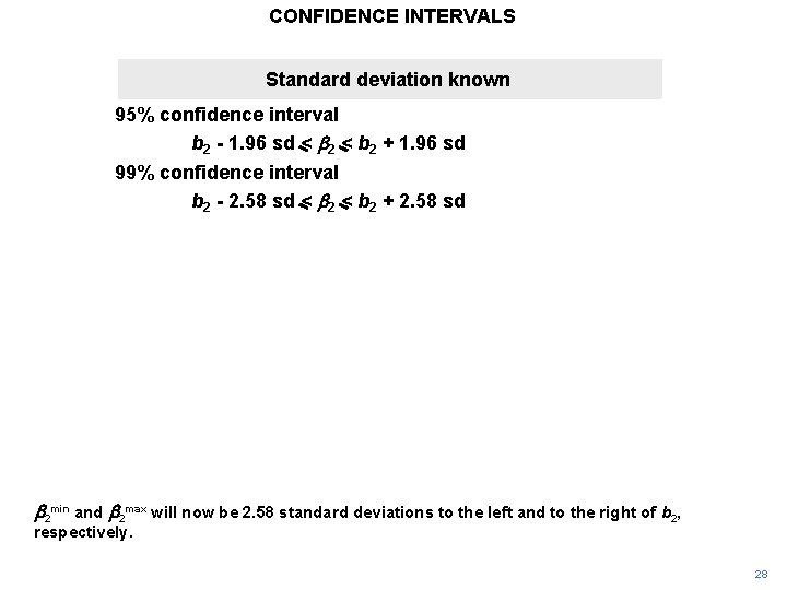
CONFIDENCE INTERVALS Standard deviation known 95% confidence interval b 2 - 1. 96 sd < b 2 + 1. 96 sd 99% confidence interval b 2 - 2. 58 sd < b 2 + 2. 58 sd b 2 min and b 2 max will now be 2. 58 standard deviations to the left and to the right of b 2, respectively. 28

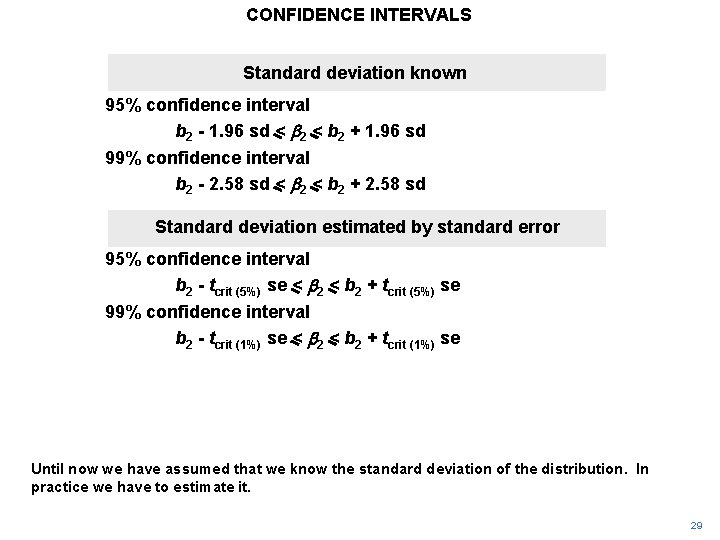
CONFIDENCE INTERVALS Standard deviation known 95% confidence interval b 2 - 1. 96 sd < b 2 + 1. 96 sd 99% confidence interval b 2 - 2. 58 sd < b 2 + 2. 58 sd Standard deviation estimated by standard error 95% confidence interval b 2 - tcrit (5%) se < b 2 + tcrit (5%) se 99% confidence interval b 2 - tcrit (1%) se < b 2 + tcrit (1%) se Until now we have assumed that we know the standard deviation of the distribution. In practice we have to estimate it. 29

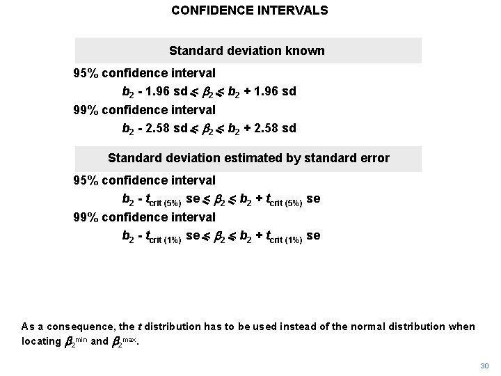
CONFIDENCE INTERVALS Standard deviation known 95% confidence interval b 2 - 1. 96 sd < b 2 + 1. 96 sd 99% confidence interval b 2 - 2. 58 sd < b 2 + 2. 58 sd Standard deviation estimated by standard error 95% confidence interval b 2 - tcrit (5%) se < b 2 + tcrit (5%) se 99% confidence interval b 2 - tcrit (1%) se < b 2 + tcrit (1%) se As a consequence, the t distribution has to be used instead of the normal distribution when locating b 2 min and b 2 max. 30

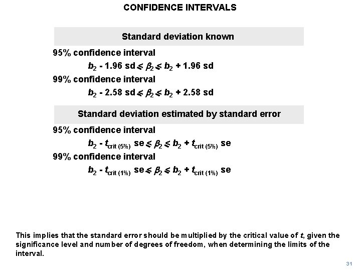
CONFIDENCE INTERVALS Standard deviation known 95% confidence interval b 2 - 1. 96 sd < b 2 + 1. 96 sd 99% confidence interval b 2 - 2. 58 sd < b 2 + 2. 58 sd Standard deviation estimated by standard error 95% confidence interval b 2 - tcrit (5%) se < b 2 + tcrit (5%) se 99% confidence interval b 2 - tcrit (1%) se < b 2 + tcrit (1%) se This implies that the standard error should be multiplied by the critical value of t, given the significance level and number of degrees of freedom, when determining the limits of the interval. 31