Confidence Intervals 10 1 Estimating a population parameter

Confidence Intervals 10. 1 “Estimating a population parameter (such as mean) based on a sample statistic (its mean)”

The value of a point estimate If all we did was to assume that = x-bar, we would be wrong 100% of the time! Close, maybe, but never right on. Why? It would be like asking, “What’s the probability in a normal distribution that x = 5? ” No can do.

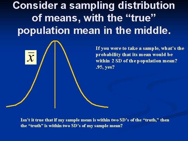
Consider a sampling distribution of means, with the “true” population mean in the middle. If you were to take a sample, what’s the probability that its mean would be within 2 SD of the population mean? . 95, yes? Isn’t it true that if my sample mean is within two SD’s of the “truth, ” then the “truth” is within two SD’s of my sample mean?

The Interval Estimate Instead of estimating the pop mean using just x-bar, now we’re going to say, “I can’t tell you for certain precisely where it is, but I can tell you that it’s likely to be within, say, two standard deviations of my x-bar. ” n Bear in mind—we’ve already established (CH 9) that the mythical x-bar distribution has the same mean as the population. n

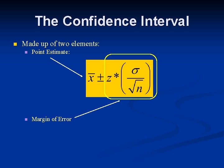
The Confidence Interval n Made up of two elements: n Point Estimate: n Margin of Error

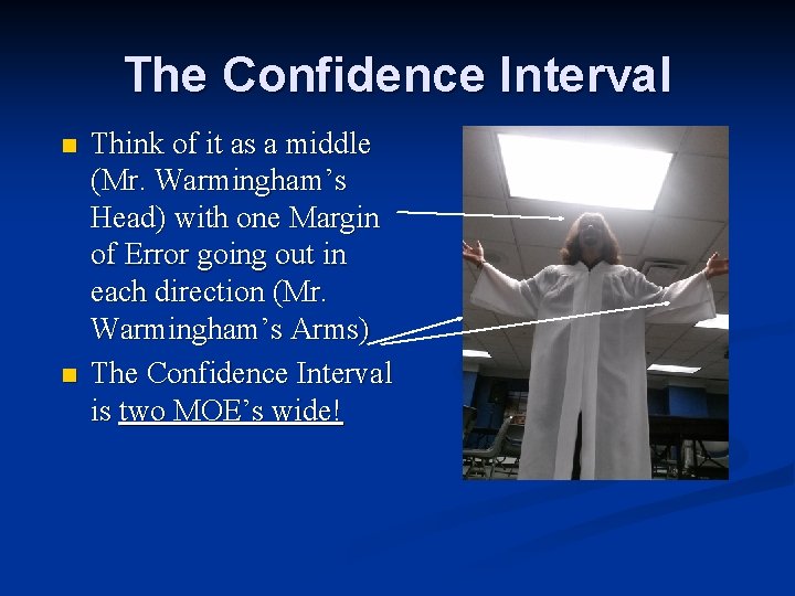
The Confidence Interval n n Think of it as a middle (Mr. Warmingham’s Head) with one Margin of Error going out in each direction (Mr. Warmingham’s Arms) The Confidence Interval is two MOE’s wide!

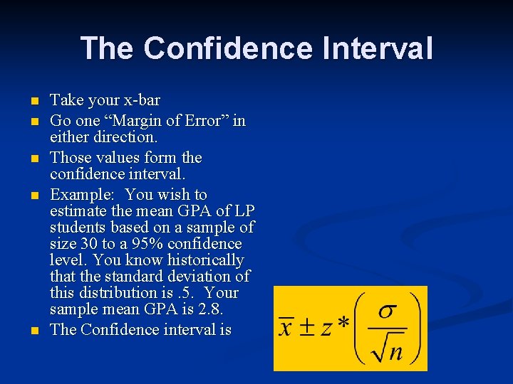
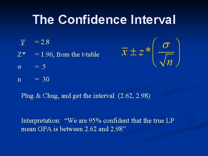
The Confidence Interval n n n Take your x-bar Go one “Margin of Error” in either direction. Those values form the confidence interval. Example: You wish to estimate the mean GPA of LP students based on a sample of size 30 to a 95% confidence level. You know historically that the standard deviation of this distribution is. 5. Your sample mean GPA is 2. 8. The Confidence interval is

Conditions or Assumptions n Conditions for a confidence interval for means: 1. Data needs to come from a Simple Random Sample n 2. The sampling distribution for means must be normal (or approximately normal). n

The Confidence Interval = 2. 8 Z* = 1. 96, from the t-table σ =. 5 n = 30 Plug & Chug, and get the interval (2. 62, 2. 98) Interpretation: “We are 95% confident that the true LP mean GPA is between 2. 62 and 2. 98”

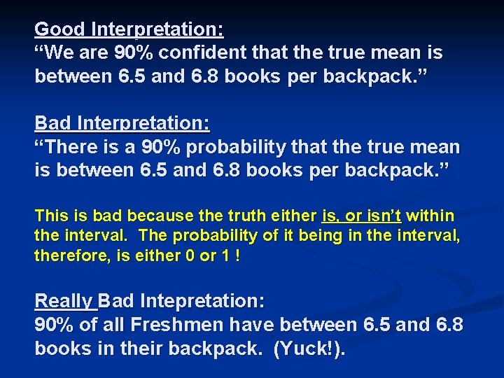
Good Interpretation: “We are 90% confident that the true mean is between 6. 5 and 6. 8 books per backpack. ” Bad Interpretation: “There is a 90% probability that the true mean is between 6. 5 and 6. 8 books per backpack. ” This is bad because the truth either is, or isn’t within the interval. The probability of it being in the interval, therefore, is either 0 or 1 ! Really Bad Intepretation: 90% of all Freshmen have between 6. 5 and 6. 8 books in their backpack. (Yuck!).

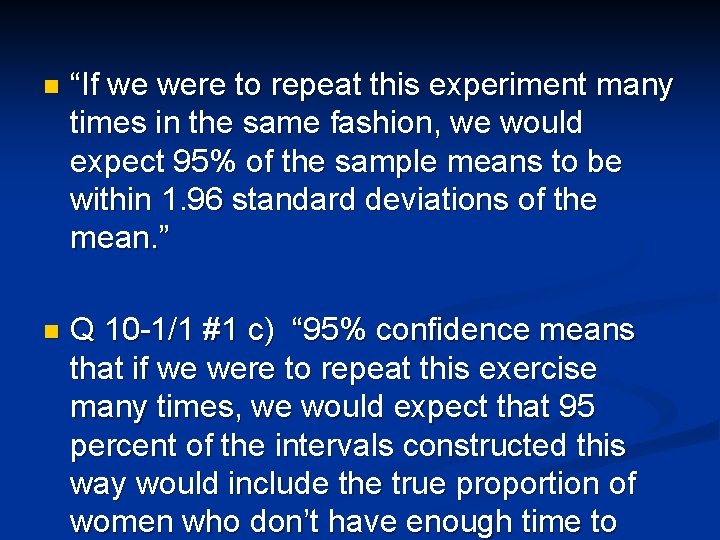
n “If we were to repeat this experiment many times in the same fashion, we would expect 95% of the sample means to be within 1. 96 standard deviations of the mean. ” n Q 10 -1/1 #1 c) “ 95% confidence means that if we were to repeat this exercise many times, we would expect that 95 percent of the intervals constructed this way would include the true proportion of women who don’t have enough time to

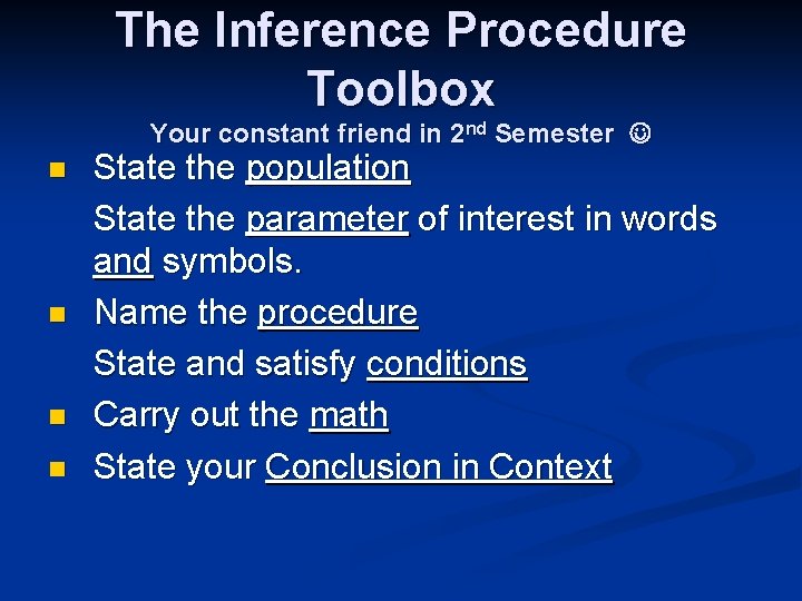
The Inference Procedure Toolbox Your constant friend in 2 nd Semester n n State the population State the parameter of interest in words and symbols. Name the procedure State and satisfy conditions Carry out the math State your Conclusion in Context

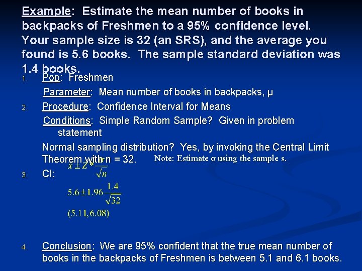
Example: Estimate the mean number of books in backpacks of Freshmen to a 95% confidence level. Your sample size is 32 (an SRS), and the average you found is 5. 6 books. The sample standard deviation was 1. 4 books. 1. 2. 3. 4. Pop: Freshmen Parameter: Mean number of books in backpacks, µ Procedure: Confidence Interval for Means Conditions: Simple Random Sample? Given in problem statement Normal sampling distribution? Yes, by invoking the Central Limit Note: Estimate σ using the sample s. Theorem with n = 32. CI: Conclusion: We are 95% confident that the true mean number of books in the backpacks of Freshmen is between 5. 1 and 6. 1 books.

Tests of Significance 10 -2 The other type of Inference Procedure (Along with Confidence Intervals)

“How Significant is this sample mean we found? ” n The basic idea: An outcome that should rarely happen if a claim were true, but that happened anyway, is strong evidence that the claim is not true. n We measure how rarely an outcome should happen using what’s called a “P-value. ” n

The P-Value n n Def: A P-Value is the probability of having found your sample mean (or one that’s more extreme), assuming the population mean is “where the Null Hypothesis says it is. ” The Null Hypothesis is the notion that: n n n Nothing’s going on There’s no meaningful change The aspirin really doesn’t reduce pain The machine really isn’t out of tolerance The stimulus really didn’t affect the economy The advertisement really didn’t help sales.

Null Hypothesis and the Scientific Method As researchers, we must always assume that the new treatment being investigated really doesn’t have any effect, i. e. that the Null Hypothesis is true, not the Alternate Hypothesis. n Only when dragged kicking and screaming by the data (or really, a low P-value) must we reject the Null Hypothesis in favor of an Alternate Hypothesis. If the evidence is not sufficient, the Null is not rejected! n

Back to P-Value and how a hypothesis test works 1. Assume Ho is true. n 2. Create a sampling distribution based on Ho and sample size n 3. Place the observed sample mean upon the sampling distribution and calculate a P -value. n 4. If that P-value is small enough, reject Ho. n

In other words… n The smaller the P-value, the less likely you are to have found such a thing… By chance alone 2. If the Null Hypothesis is true. The P-value we’ve got to be below is called α if we want to reject Ho. This is called a significance level. Say someone declares α to be. 05. You produce a p-value of. 04. We’d say “Reject Ho at the. 05 significance level. ” 1. n n

Where do low P-Values come from? 1. 2. 3. Three possibilities Mere chance (bad research luck, in other words—unlikely) Bad Sampling Wrong Ho! By insisting on a low P-value, the first is unlikely. By insisting on an SRS, the second is controlled.

“If the P is low, the Ho must go!”

“If the P is low, the Ho must go!” A result that causes us to reject Ho we call “statistically significant. ” It’s a finding* so rare that chance alone would very seldom produce it. Because it happened anyway, it probably wasn’t mere chance that caused it! * A sample mean, for example

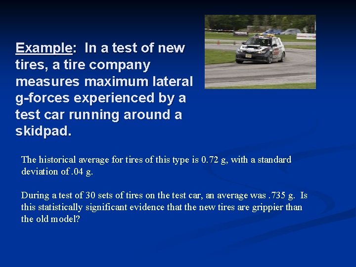
Example: In a test of new tires, a tire company measures maximum lateral g-forces experienced by a test car running around a skidpad. The historical average for tires of this type is 0. 72 g, with a standard deviation of. 04 g. During a test of 30 sets of tires on the test car, an average was. 735 g. Is this statistically significant evidence that the new tires are grippier than the old model?

A Toolbox! Yea! n Step 1: Population: Tires of this new type n Parameter: Average maximum g-forces, µ n Ho: The average of this new type is just like the old. µ =. 72 n Ha: The average for this new tire is greater than the old. µ >. 72 n

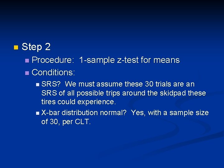
n Step 2 Procedure: 1 -sample z-test for means n Conditions: n n SRS? We must assume these 30 trials are an SRS of all possible trips around the skidpad these tires could experience. n X-bar distribution normal? Yes, with a sample size of 30, per CLT.

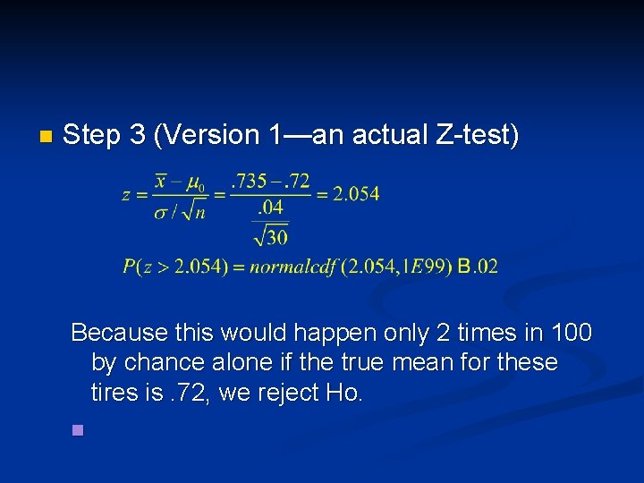
n Step 3 (Version 1—an actual Z-test) Because this would happen only 2 times in 100 by chance alone if the true mean for these tires is. 72, we reject Ho. n

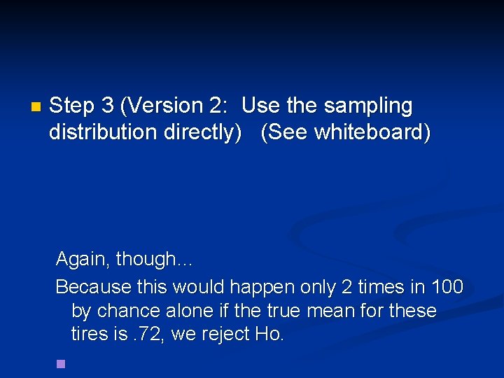
n Step 3 (Version 2: Use the sampling distribution directly) (See whiteboard) Again, though… Because this would happen only 2 times in 100 by chance alone if the true mean for these tires is. 72, we reject Ho. n

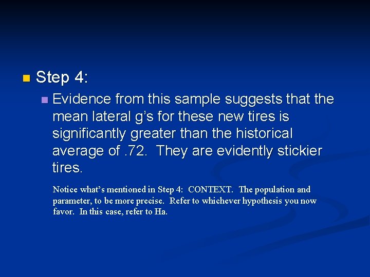
n Step 4: n Evidence from this sample suggests that the mean lateral g’s for these new tires is significantly greater than the historical average of. 72. They are evidently stickier tires. Notice what’s mentioned in Step 4: CONTEXT. The population and parameter, to be more precise. Refer to whichever hypothesis you now favor. In this case, refer to Ha.

An unfortunate non-sequitur n Common mistake by students: n “Step 4: The tires are significantly sticker. Therefore we reject Ho. ” Yuck! Cart before horse! Your conclusion is a consequence of having rejected Ho—not vice versa. And besides, never finish an inference procedure with your reject/fail to reject statement. Finish with your conclusion in

Choosing α and Statistical vs. real significance 10 -3 Don’t blink. This goes quickly.

Choosing significance level n Consider two main things when deciding whether to go with a more relaxed α (. 05) or a more stringent α (. 01, . 001). n n n How much “convincing” is necessary for your purpose. (Who’s your audience? How expensive or costly would be the consequence of rejecting Ho. If rejecting Ho would be costly in dollars, lives, careers, you’d better require your findings to climb a tall mountain. (a small α) IRL, α level isn’t all that important. p =. 048 is not that different than p =. 052.

Statistical vs. Real-life Significance n “We’re thrilled you’ve got a small P-value, but so what? ” n n Not all findings—though they reach statistical significance—really matter. See Example 10. 18 on p. 588.

Small P-Values don’t fix bad sampling Don’t shout Eureka until you’re sure your sampling & methodology is correct. n In fact, your small p-value may be precisely because of cheesy sampling. Sometimes your small p-value is evidence that you messed up! n

10 -4 (Get tough—this one’s chewy) n Type 1 Error: Rejecting Ho when you really shouldn’t have. n Example: You replace all the bearings in a piece of manufacturing equipment, but afterwards the machine is still pretty sloppy. n Example: A jury finds a defendant “not guilty. ” (Ho was “Not Guilty” and they failed to reject it). Later, a new witness comes forth and provides evidence that the guy really did do the crime!.

10 -4 n Type 2 Error: Failing to Reject Ho when you really should have! Example: Ho: Student doesn’t know the material for a test. Test score is low, so teacher gives student an F. Later it’s found that the student is strongly dyslexic, and was unable to properly choose among multiplechoice answers. n Example: A jury rejects Ho (Ho was “Not Guilty”) and convicts a defendant. Later, DNA evidence reveals the defendant couldn’t have n