Conceptual Model A descriptive representation of a groundwater

Conceptual Model A descriptive representation of a groundwater system that incorporates an interpretation of the geological & hydrological conditions. Generally includes information about the water budget. May include information on water chemistry.

Mathematical Model a set of equations that describes the physical and/or chemical processes occurring in a system.

Derivation of the Governing Equation Q R x y q z x y 1. Consider flux (q) through REV 2. OUT – IN = - Storage 3. Combine with: q = -K grad h

General 3 D equation 2 D confined: 2 D unconfined w/ Dupuit assumptions: Storage coefficient (S) is either storativity or specific yield. S = Ss b & T = K b

Types of Boundary Conditions 1. Specified head 2. Specified flow (including no flow) 3. Head-dependent flow

From conceptual model to mathematical model…

Toth Problem Water table forms the upper boundary condition h = c x + zo Laplace Equation 2 D, steady state Cross section through an unconfined aquifer.

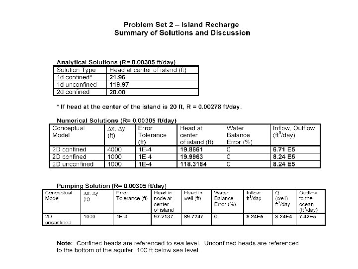
“Confined” Island Recharge Problem We can treat this system as a “confined” aquifer if we assume that T= Kb. Areal view Water table is the solution. R h groundwater divide ocean Poisson’s Eqn. ocean b x=-L datum x=0 x=L 2 D horizontal flow through an unconfined aquifer where T=Kb.

Unconfined version of the Island Recharge Problem (Pumping can be accommodated by appropriate definition of the source/sink term. ) Water table is the solution. R groundwater divide ocean b datum x=-L h ocean x=0 x=L 2 D horizontal flow through an unconfined aquifer under the Dupuit assumptions.

Vertical cross section through an unconfined aquifer with the water table as the upper boundary. 2 D horizontal flow in a confined aquifer; solution is h(x, y), i. e. , the potentiometric surface. 2 D horizontal flow in an unconfined aquifer where v= h 2. Solution is h(x, y), i. e. , the water table. All three governing equations are the La. Place Eqn.

Reservoir Problem t=0 t>0 datum 0 L = 100 m BC: h (0, t) = 16 m; t > 0 h (L, t) = 11 m; t > 0 IC: h (x, 0) = 16 m; 0 < x < L (represents static steady state) 1 D transient flow through a confined aquifer. x

Solution techniques…

Three options: • Iteration • Direct solution by matrix inversion • A combination of iteration and matrix solution

Examples of Iteration methods include: Gauss-Seidel Iteration Successive Over-Relaxation (SOR)

Let x= y=a

Gauss-Seidel Formula for 2 D Laplace Equation General SOR Formula Relaxation factor = 1 Gauss-Seidel < 1 under-relaxation >1 over-relaxation, typically between 1 and 2 (e. g. , 1. 8)

Gauss-Seidel Formula for 2 D Poisson Equation (Eqn. 3. 7 W&A) SOR Formula Relaxation factor = 1 Gauss-Seidel < 1 under-relaxation >1 over-relaxation

solution Iteration for a steady state problem. m+3 Iteration levels m+2 m+1 m (Initial guesses)

Transient Problems require time steps. Steady state n+3 t n+2 Time levels t n+1 t n Initial conditions (at steady state)

Explicit Approximation Implicit Approximation Or weighted average

• Explicit solutions do not require iteration but are unstable with large time steps. • We can derive the stability criterion by writing the explicit approx. in a form that looks like the SOR iteration formula and setting the terms in the position occupied by omega equal to 1. • For the 1 D governing equation used in the reservoir problem, the stability criterion is: < or <

Implicit solutions require iteration or direct solution by matrix inversion.

n+1 t m+3 m+2 Iteration planes m+1 n Solution by iteration

Modeling “Rules” • Boundary conditions always affect a steady state solution. • Initial conditions should be selected to represent a steady state configuration of heads.