COMSOL Multiphysics Conference 2005 Cambridge MA Oct 24

COMSOL Multiphysics Conference 2005, Cambridge, MA Oct 24, 2005 S-Parameter Sensitivity Analysis of Waveguide Structures with COMSOL Multiphysics Dongying Li and N. K. Nikolova (e-mail: lid 6@mcmaster. ca) Mc. Master University, 1280 Main Street West, Hamilton, ON L 8 S 4 K 1, CANADA Department of Electrical and Computer Engineering Computational Electromagnetics Laboratory

Contents • Theory • Implementation in COMSOL Multiphysics • Numerical Results

Theory Sensitivity Analysis: Given: 1. The FEM system equation: 2. Design variables 3. Objective function Find the function gradient equation subject to the system While in S-parameter sensitivity analysis:

Applications of sensitivity analysis 1. Gradient based optimization: 2. Yield and tolerance analysis

Traditional method Finite-difference method at the response level:
 for FEM For FEM formulation We have the adjoint variable")
Adjoint variable method (AVM) for FEM For FEM formulation We have the adjoint variable formula according to the ith design parameter is the solution vector of the adjoint system equation:

Self-adjoint sensitivity analysis method on S-parameters The solution of the S-parameter usually has no explicit dependent on p and is not related to the excitation vector b. The AVM sensitivity formula can be written as:

Self-adjoint sensitivity analysis method on S-parameters By the self-adjoint nature of the S-parameter problem, we can find a linear relationship between the k-th element of the original excitation vector and the adjoint excitation vector: For Finite-element formulation:

Self-adjoint sensitivity analysis method on S-parameters A linear relationship between the elements of the original solution vector and the adjoint solution vector exists: And the AVM formulation becomes

Computational cost comparison For the S-parameter sensitivity analysis of an M-port microwave structure with n design parameters FD AVM SASA Original system analysis M M M Additional system analysis M*n (perturbed) M (adjoint) 0 total M*(n+1) 2 M M

Implementation in COMSOL Multiphysics • • Basic procedure to perform a self-adjoint sensitivity analysis: Build the geometric and physical model. Generate mesh. Solve the system equation, compute the original S-parameters. Record the solution vector x and the system matrix. Perturb the structure and rebuild the perturbed mesh. Assemble the system matrix on perturbed structure and compute the derivative of system matrix. Compute the self-adjoint sensitivity formula, using the derivative of system matrix and solution vector.

Two requirement for the FEM solver : 1. The system matrix must be exportable. 2. The system matrix on the original and the perturbed problem must be the same size, thus the unstructured mesh must be able to be manipulated manually. COMSOL Multiphysics can satisfactorily meet the requirements through its MATLAB interface functions.
![fem. mesh = meshinit(fem); fem. xmesh = meshextend(fem); [Kl Ll] = femlin(fem, 'out', {'Kl'](http://slidetodoc.com/presentation_image_h2/a11db67992c625f948d7359998d67343/image-13.jpg "fem. mesh = meshinit(fem); fem. xmesh = meshextend(fem); [Kl Ll] = femlin(fem, 'out', {'Kl'")
fem. mesh = meshinit(fem); fem. xmesh = meshextend(fem); [Kl Ll] = femlin(fem, 'out', {'Kl' 'Ll'}); x = Kl Ll; … p = fem. mesh. p; el = get(fem. mesh, 'el'); <alter the mesh> … fem_perturb. mesh = femmesh(p_purturb, el); … [Kl_perturb Ll] = femlin(fem_purturb, 'out', {'Kl' 'Ll'}); d. K = (Kl_purturb – Kl) / dp;

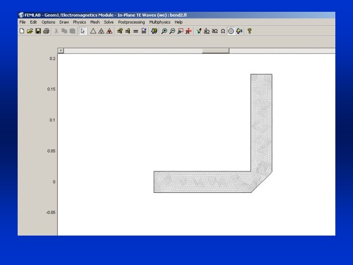
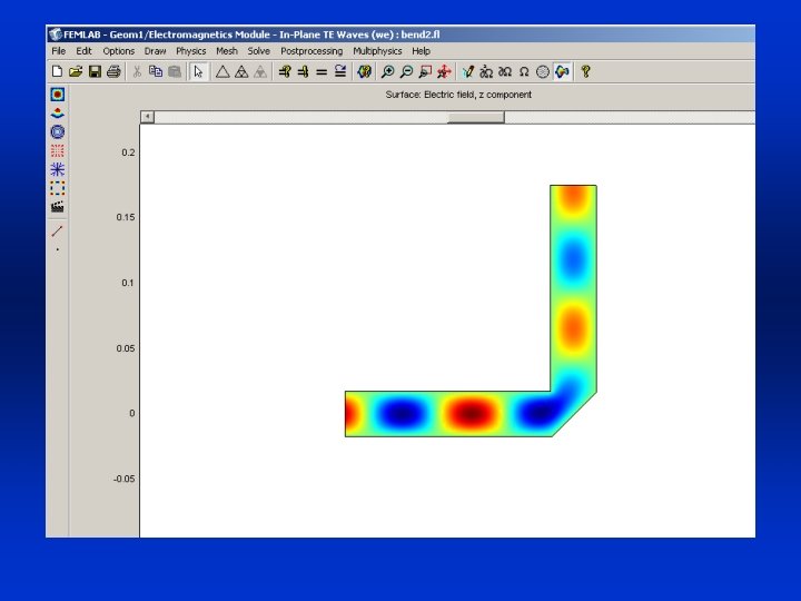
Numerical Examples waveguide bend


Thank you Question?
- Slides: 18