Computing Gradient Hungyi Lee Introduction Backpropagation an efficient

Computing Gradient Hung-yi Lee 李宏毅

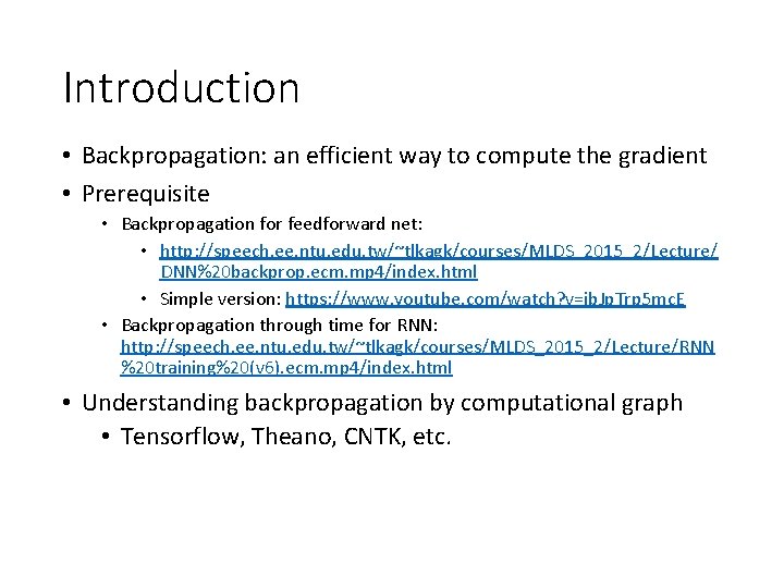
Introduction • Backpropagation: an efficient way to compute the gradient • Prerequisite • Backpropagation for feedforward net: • http: //speech. ee. ntu. edu. tw/~tlkagk/courses/MLDS_2015_2/Lecture/ DNN%20 backprop. ecm. mp 4/index. html • Simple version: https: //www. youtube. com/watch? v=ib. Jp. Trp 5 mc. E • Backpropagation through time for RNN: http: //speech. ee. ntu. edu. tw/~tlkagk/courses/MLDS_2015_2/Lecture/RNN %20 training%20(v 6). ecm. mp 4/index. html • Understanding backpropagation by computational graph • Tensorflow, Theano, CNTK, etc.

Computational Graph

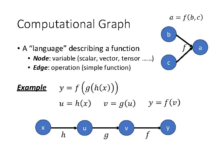
Computational Graph b a • A “language” describing a function • Node: variable (scalar, vector, tensor ……) • Edge: operation (simple function) c Example x u v y

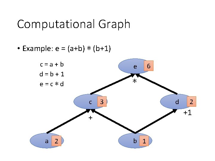
Computational Graph • Example: e = (a+b) ∗ (b+1) c=a+b d=b+1 e=c∗d e ∗ c 3 d 2 +1 + a 2 6 b 1

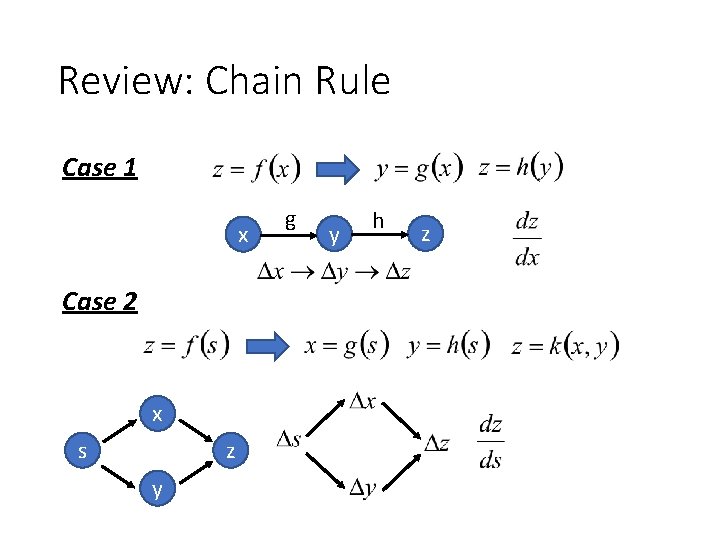
Review: Chain Rule Case 1 x Case 2 x s z y g y h z

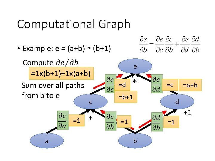
Computational Graph • Example: e = (a+b) ∗ (b+1) =1 x(b+1)+1 x(a+b) Sum over all paths from b to e c =1 a + e =d ∗ =c =b+1 =a+b d +1 =1 =1 b

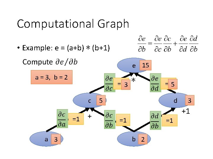
Computational Graph • Example: e = (a+b) ∗ (b+1) e 15 a = 3, b = 2 =d 3 ∗ c =1 a 3 + =c 5 5 d 3 +1 =1 =1 b 2

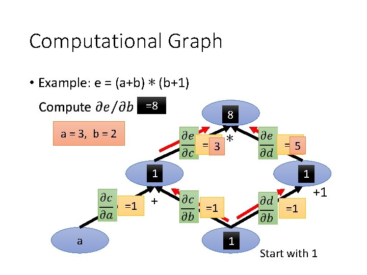
Computational Graph • Example: e = (a+b) ∗ (b+1) =8 a = 3, b = 2 8 e =d 3 ∗ =c 5 1 c =1 a + d 1 +1 =1 =1 b 1 Start with 1

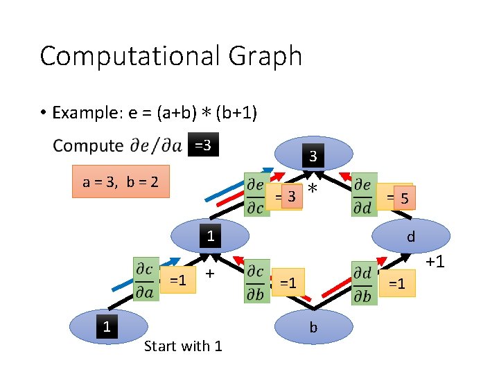
Computational Graph • Example: e = (a+b) ∗ (b+1) =3 a = 3, b = 2 3 e =d 3 ∗ =c 5 1 c =1 1 a + Start with 1 d +1 =1 =1 b

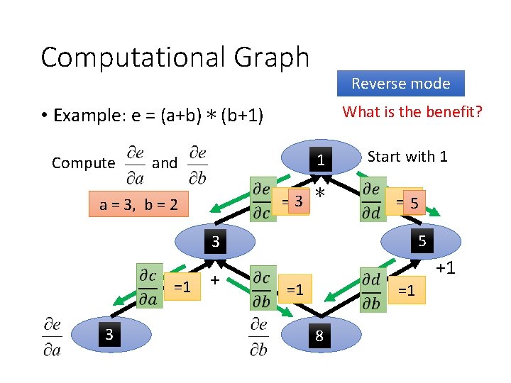
Computational Graph Reverse mode What is the benefit? • Example: e = (a+b) ∗ (b+1) and 1 e a = 3, b = 2 =d 3 ∗ Compute Start with 1 =c 5 d 5 3 c =1 3 a + +1 =1 =1 8 b

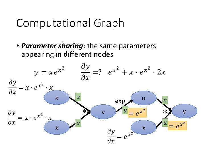
Computational Graph • Parameter sharing: the same parameters appearing in different nodes x exp ∗ x u ∗ v x y

Computational Graph for Feedforward Net

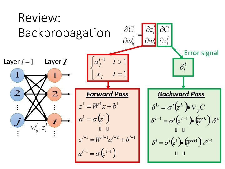
Review: Backpropagation Layer Error signal Layer Forward Pass Backward Pass … …

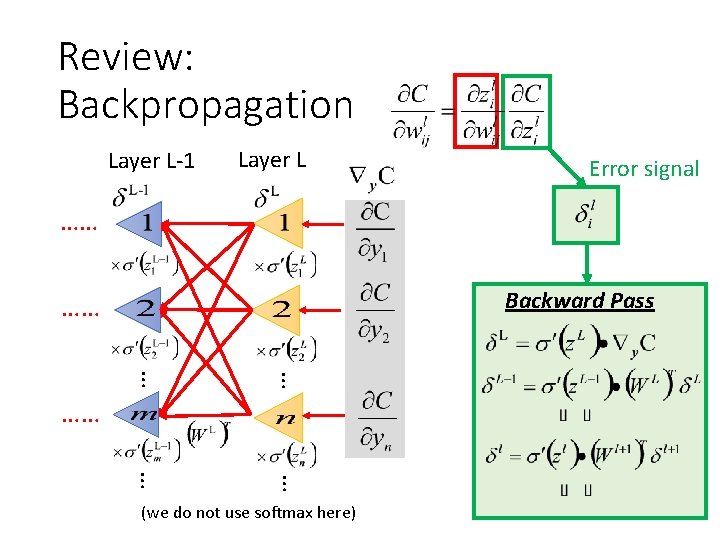
Review: Backpropagation Layer L-1 Layer L Error signal …… Backward Pass …… … … …… (we do not use softmax here)

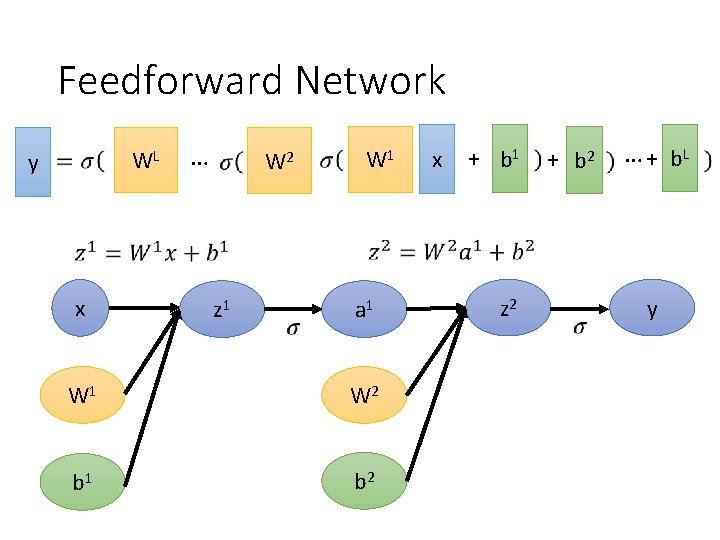
Feedforward Network WL y x … W 2 z 1 W 1 a 1 W 2 b 1 b 2 x + b 1 z 2 + b 2 … + b. L y

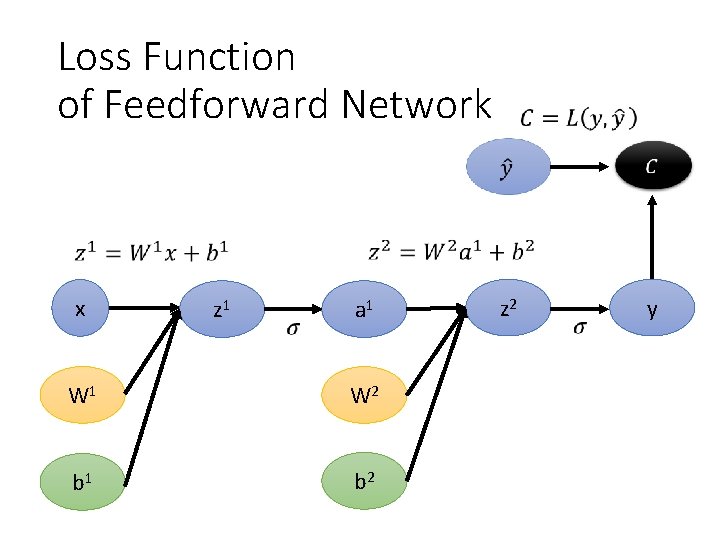
Loss Function of Feedforward Network x z 1 a 1 W 2 b 1 b 2 z 2 y

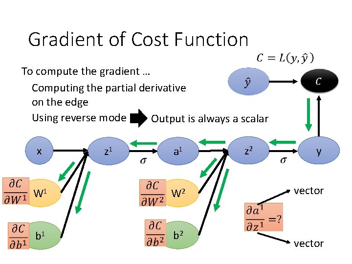
Gradient of Cost Function To compute the gradient … Computing the partial derivative on the edge Using reverse mode Output is always a scalar x z 1 a 1 W 2 b 1 b 2 z 2 y vector

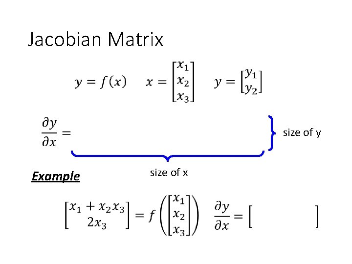
Jacobian Matrix size of y Example size of x

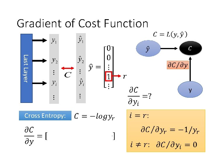
Gradient of Cost Function … … Last Layer … … Cross Entropy: y

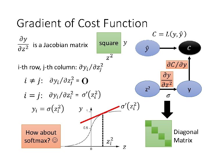
Gradient of Cost Function is a Jacobian matrix square z 2 How about softmax? y Diagonal Matrix

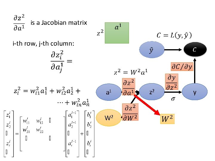
is a Jacobian matrix i-th row, j-th column: a 1 W 2 z 2 y

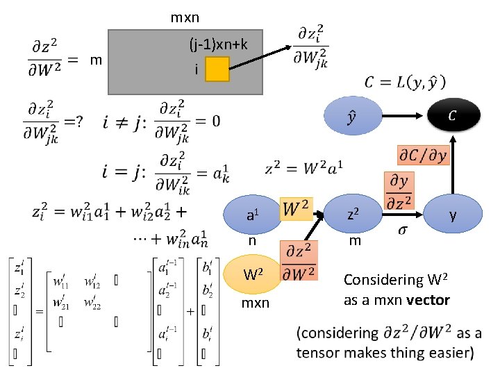
mxn m (j-1)xn+k i y a 1 n z 2 W 2 Considering W 2 as a mxn vector mxn m

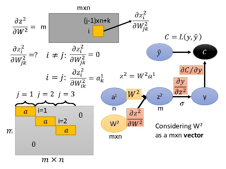
mxn (j-1)xn+k i m i=1 i=2 y a 1 n z 2 W 2 Considering W 2 as a mxn vector mxn m

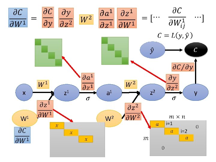
x W 1 z 1 a 1 W 2 z 2 y

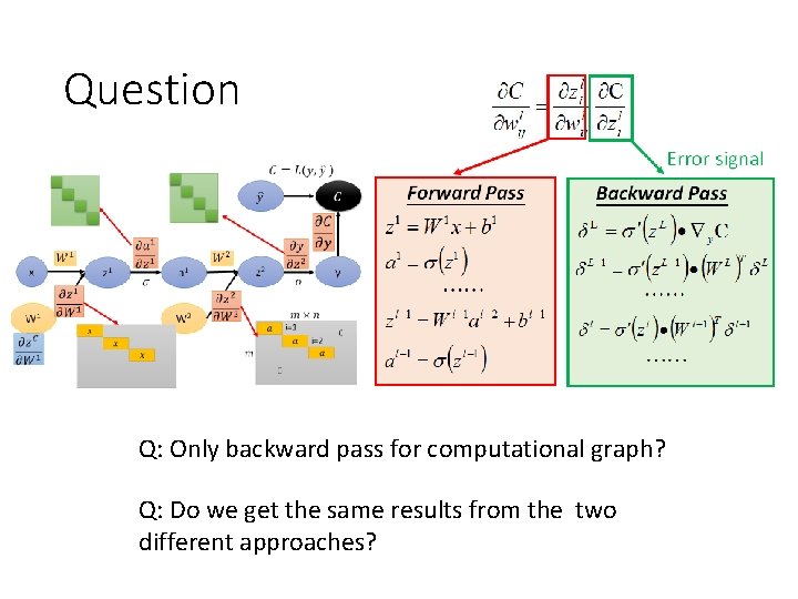
Question Q: Only backward pass for computational graph? Q: Do we get the same results from the two different approaches?

Computational Graph for Recurrent Network

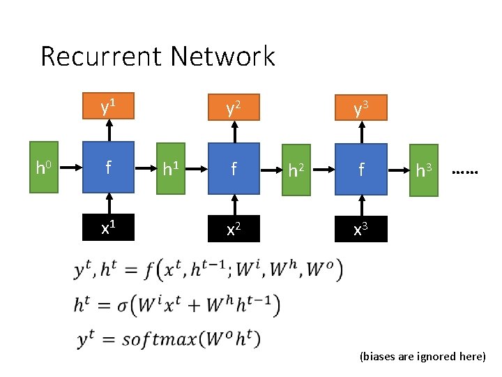
Recurrent Network y 1 h 0 f x 1 y 2 h 1 f x 2 y 3 h 2 f h 3 …… x 3 (biases are ignored here)

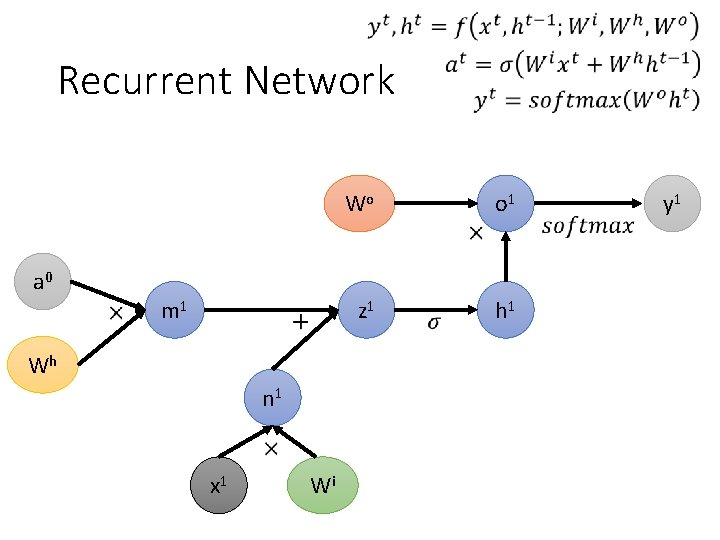
Recurrent Network a 0 m 1 Wh n 1 x 1 Wi Wo o 1 z 1 h 1 y 1

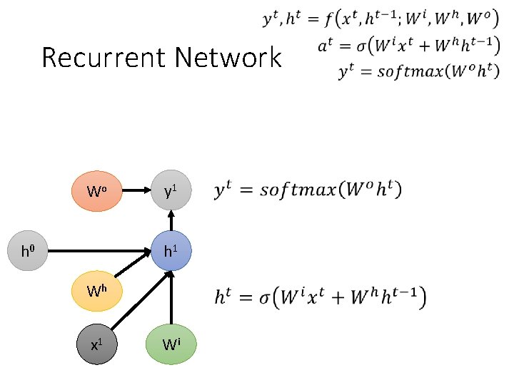
Recurrent Network Wo h 0 y 1 h 1 Wh x 1 Wi

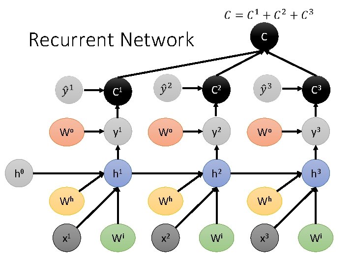
Recurrent Network C 2 C 1 Wo h 0 y 1 Wo h 1 Wh x 1 C y 2 Wo h 2 Wh Wi C 3 x 2 y 3 h 3 Wh Wi x 3 Wi

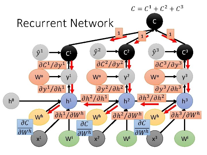
Recurrent Network h 0 y 1 Wo h 1 Wh x 1 1 y 2 C 3 Wo h 2 Wh Wi 1 1 C 2 C 1 Wo C x 2 y 3 h 3 Wh Wi x 3 Wi

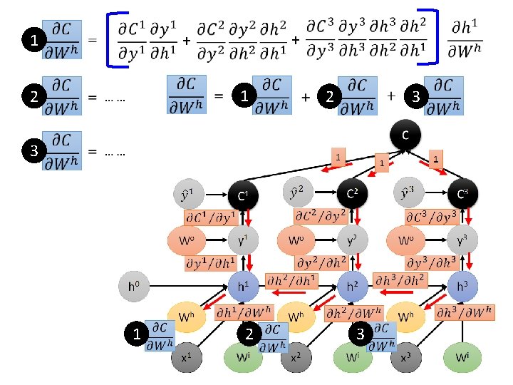
1 + + 1 2 2 3 3 1 2 3

Reference • Textbook: Deep Learning • Chapter 6. 5 • Calculus on Computational Graphs: Backpropagation • https: //colah. github. io/posts/2015 -08 Backprop/ • On chain rule, computational graphs, and backpropagation • http: //outlace. com/Computational-Graph/