Computer Vision TP 7 Segmentation Miguel Tavares Coimbra

Computer Vision – TP 7 Segmentation Miguel Tavares Coimbra

Outline • Introduction to segmentation • Thresholding • Region based segmentation Computer Vision - TP 7 - Segmentation 2

Topic: Introduction to segmentation • Thresholding • Region based segmentation Computer Vision - TP 7 - Segmentation 3

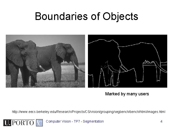
Boundaries of Objects Marked by many users http: //www. eecs. berkeley. edu/Research/Projects/CS/vision/grouping/segbench/html/images. html Computer Vision - TP 7 - Segmentation 4

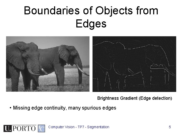
Boundaries of Objects from Edges Brightness Gradient (Edge detection) • Missing edge continuity, many spurious edges Computer Vision - TP 7 - Segmentation 5

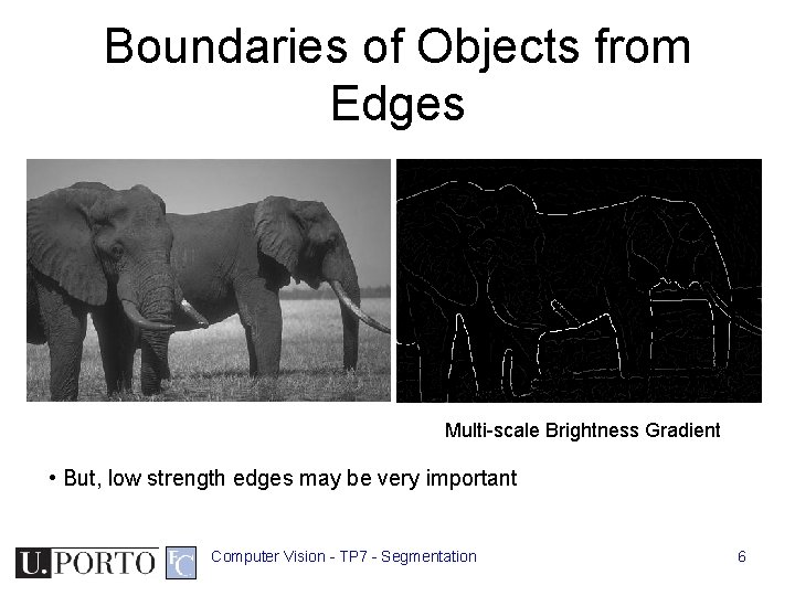
Boundaries of Objects from Edges Multi-scale Brightness Gradient • But, low strength edges may be very important Computer Vision - TP 7 - Segmentation 6

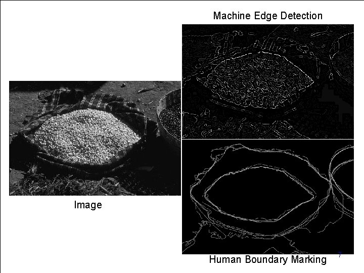
Machine Edge Detection Image Computer Vision - TP 7 - Segmentation Human Boundary Marking 7

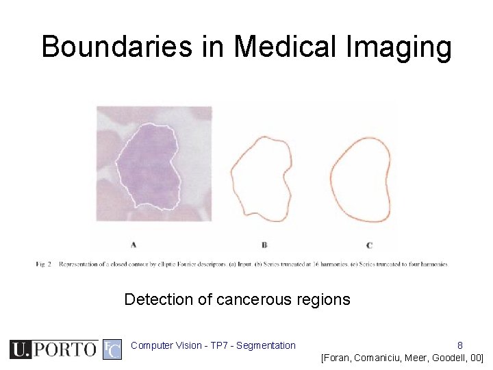
Boundaries in Medical Imaging Detection of cancerous regions Computer Vision - TP 7 - Segmentation 8 [Foran, Comaniciu, Meer, Goodell, 00]

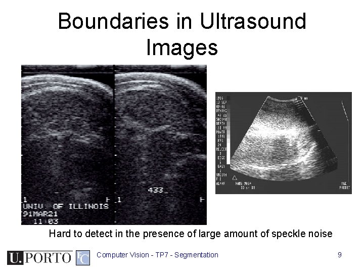
Boundaries in Ultrasound Images Hard to detect in the presence of large amount of speckle noise Computer Vision - TP 7 - Segmentation 9

Computer Vision - TP 7 - Segmentation Sometimes hard even for humans! 10

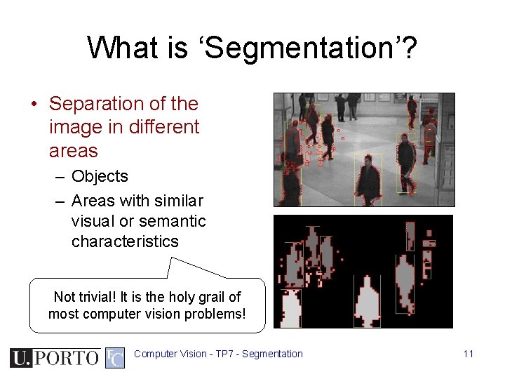
What is ‘Segmentation’? • Separation of the image in different areas – Objects – Areas with similar visual or semantic characteristics Not trivial! It is the holy grail of most computer vision problems! Computer Vision - TP 7 - Segmentation 11

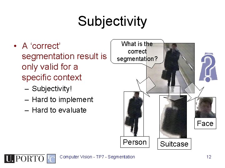
Subjectivity • A ‘correct’ segmentation result is only valid for a specific context What is the correct segmentation? – Subjectivity! – Hard to implement – Hard to evaluate Face Person Computer Vision - TP 7 - Segmentation Suitcase 12

Topic: Thresholding • Introduction to segmentation • Thresholding • Region based segmentation Computer Vision - TP 7 - Segmentation 13

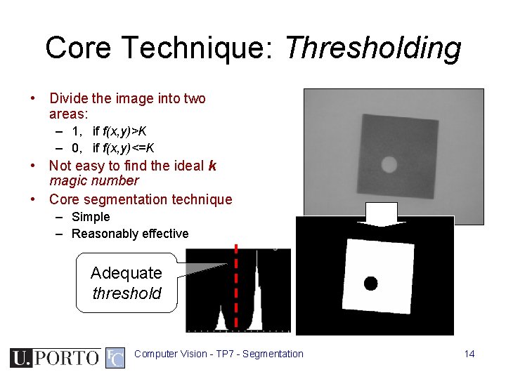
Core Technique: Thresholding • Divide the image into two areas: – 1, if f(x, y)>K – 0, if f(x, y)<=K • Not easy to find the ideal k magic number • Core segmentation technique – Simple – Reasonably effective Adequate threshold Computer Vision - TP 7 - Segmentation 14

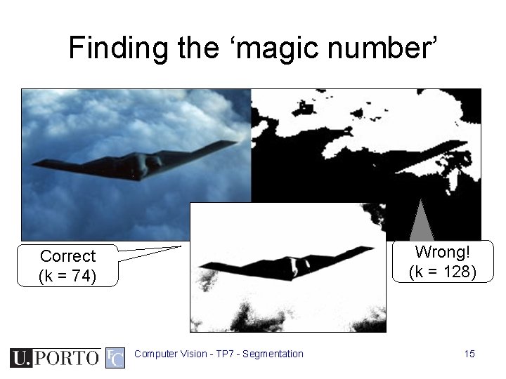
Finding the ‘magic number’ Wrong! (k = 128) Correct (k = 74) Computer Vision - TP 7 - Segmentation 15

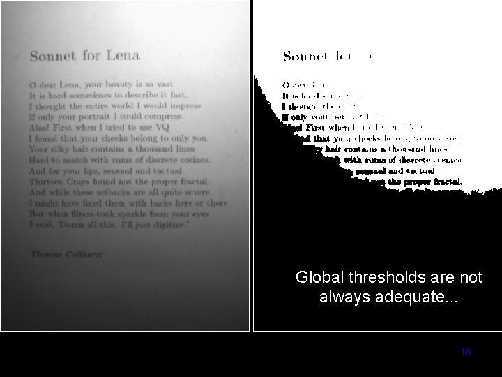
Global thresholds are not always adequate. . . Computer Vision - TP 7 - Segmentation 16

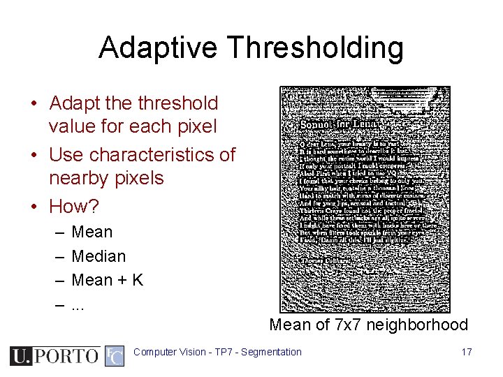
Adaptive Thresholding • Adapt the threshold value for each pixel • Use characteristics of nearby pixels • How? – – Mean Median Mean + K . . . Mean of 7 x 7 neighborhood Computer Vision - TP 7 - Segmentation 17

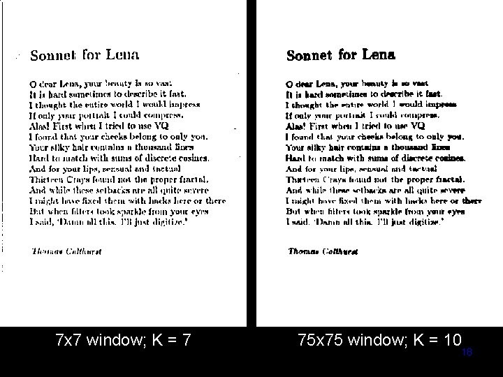
7 x 7 window; K = 7 75 x 75 window; K = 10 Computer Vision - TP 7 - Segmentation 18

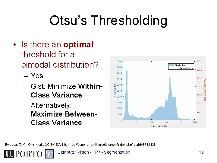
Otsu’s Thresholding • Is there an optimal threshold for a bimodal distribution? – Yes – Gist: Minimize Within. Class Variance – Alternatively: Maximize Between. Class Variance By Lucas(CA) - Own work, CC BY-SA 4. 0, https: //commons. wikimedia. org/w/index. php? curid=67144384 Computer Vision - TP 7 - Segmentation 19

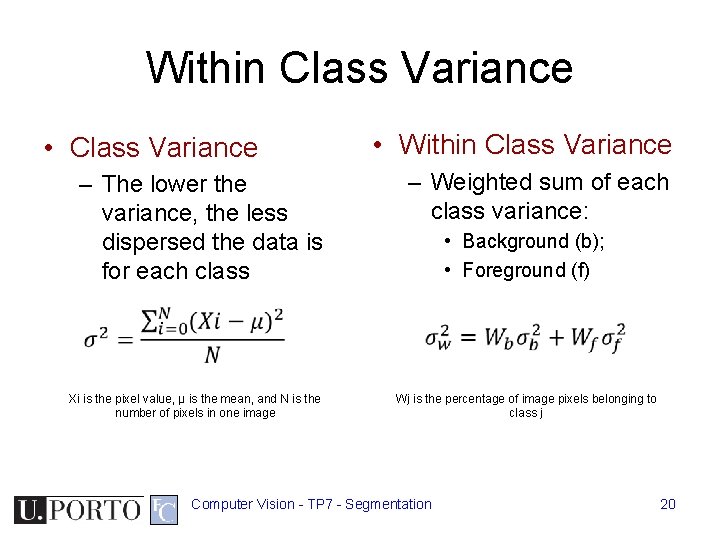
Within Class Variance • Class Variance – The lower the variance, the less dispersed the data is for each class • Within Class Variance – Weighted sum of each class variance: • Background (b); • Foreground (f) Xi is the pixel value, μ is the mean, and N is the number of pixels in one image Wj is the percentage of image pixels belonging to class j Computer Vision - TP 7 - Segmentation 20

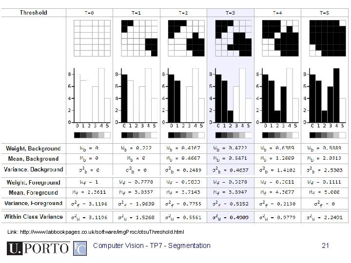
Link: http: //www. labbookpages. co. uk/software/img. Proc/otsu. Threshold. html Computer Vision - TP 7 - Segmentation 21

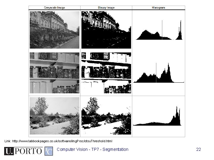
Link: http: //www. labbookpages. co. uk/software/img. Proc/otsu. Threshold. html Computer Vision - TP 7 - Segmentation 22

Topic: Region based segmentation • Introduction to segmentation • Thresholding • Region based segmentation Computer Vision - TP 7 - Segmentation 23

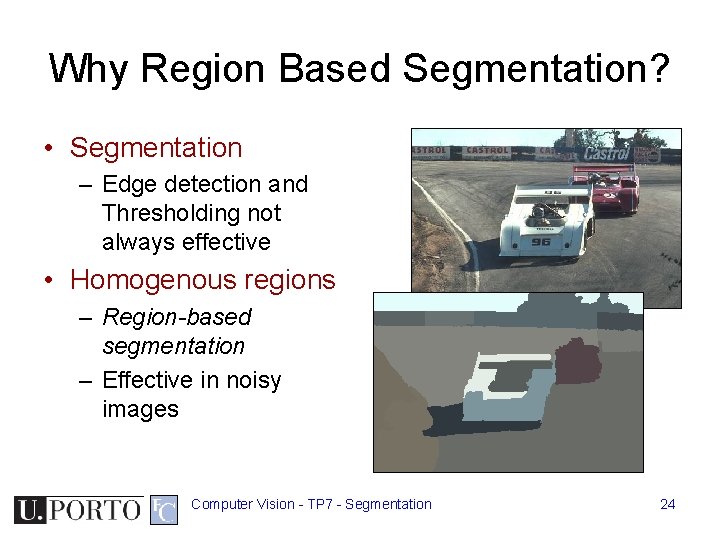
Why Region Based Segmentation? • Segmentation – Edge detection and Thresholding not always effective • Homogenous regions – Region-based segmentation – Effective in noisy images Computer Vision - TP 7 - Segmentation 24

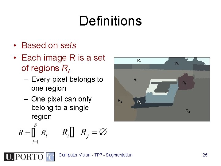
Definitions • Based on sets • Each image R is a set of regions Ri – Every pixel belongs to one region – One pixel can only belong to a single region R 7 R 1 R 2 Computer Vision - TP 7 - Segmentation R 6 R 5 R 3 R 4 25

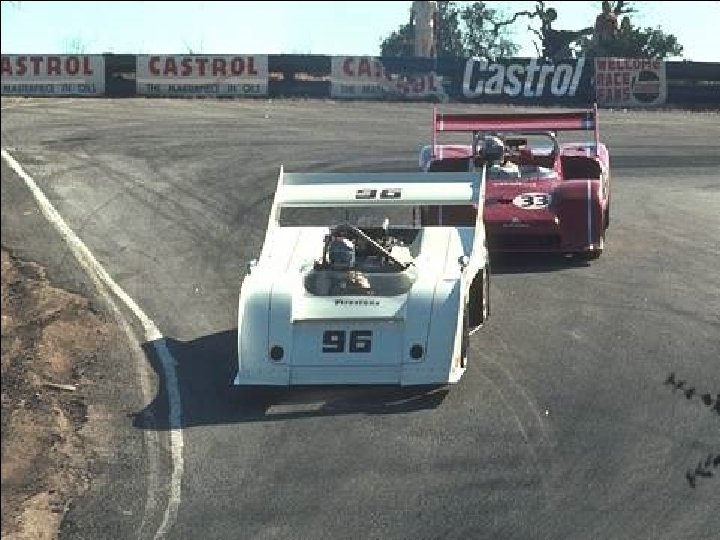
Computer Vision - TP 7 - Segmentation 26

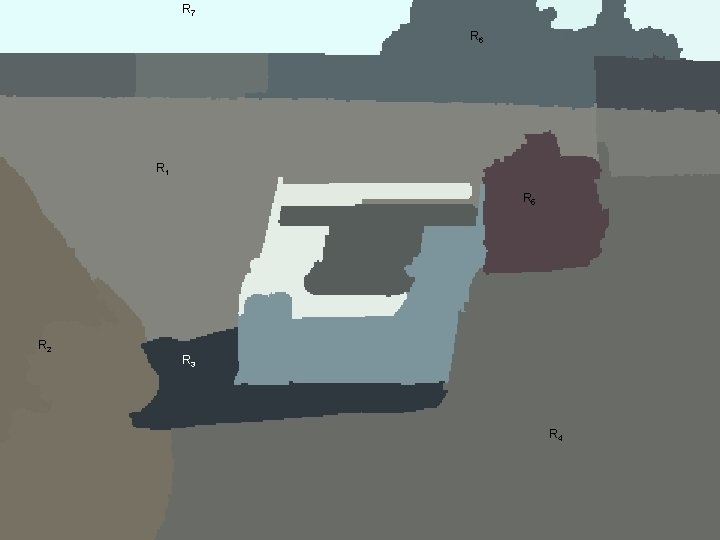
R 7 R 6 R 1 R 5 R 2 R 3 R 4 Computer Vision - TP 7 - Segmentation 27

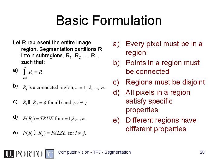
Basic Formulation Let R represent the entire image region. Segmentation partitions R into n subregions, R 1, R 2, . . . , Rn, such that: a) b) c) d) e) a) Every pixel must be in a region b) Points in a region must be connected c) Regions must be disjoint d) All pixels in a region satisfy specific properties e) Different regions have different properties Computer Vision - TP 7 - Segmentation 28

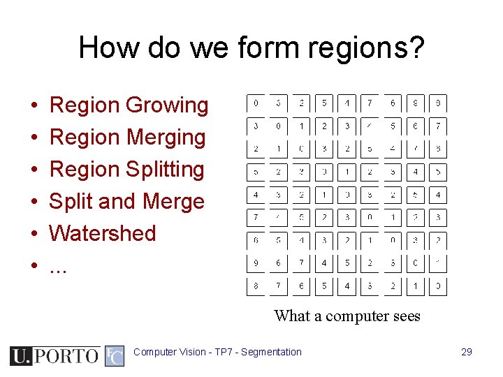
How do we form regions? • • • Region Growing Region Merging Region Splitting Split and Merge Watershed. . . What a computer sees Computer Vision - TP 7 - Segmentation 29

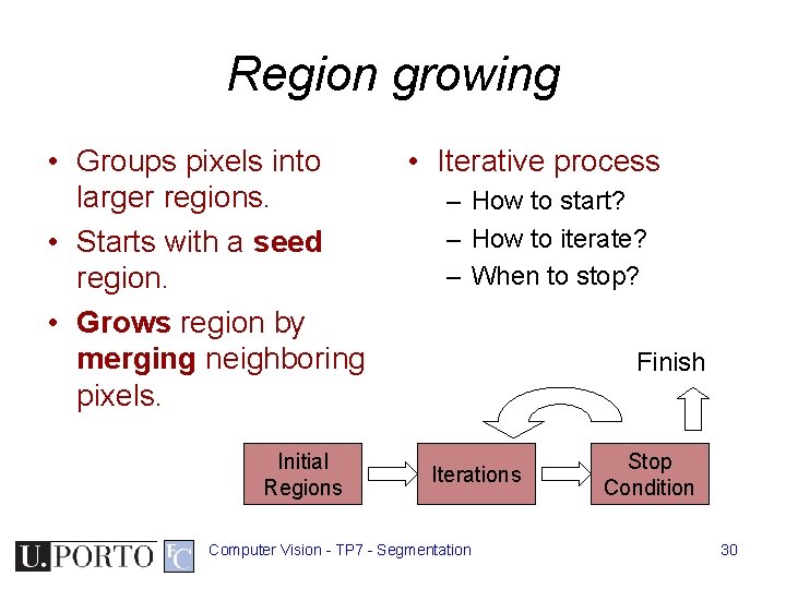
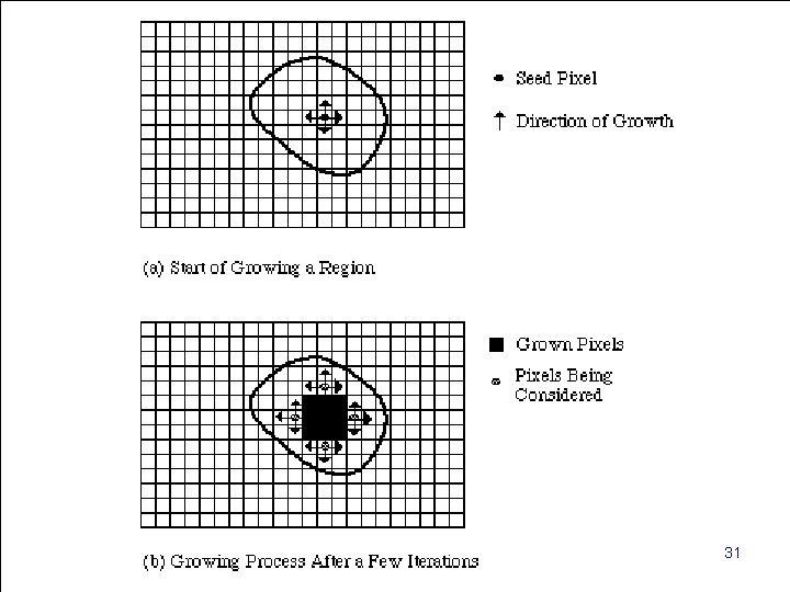
Region growing • Groups pixels into larger regions. • Starts with a seed region. • Grows region by merging neighboring pixels. Initial Regions • Iterative process – How to start? – How to iterate? – When to stop? Finish Iterations Computer Vision - TP 7 - Segmentation Stop Condition 30

Computer Vision - TP 7 - Segmentation 31

Region merging • Algorithm – Divide image into an initial set of regions • One region per pixel – Define a similarity criteria for merging regions – Merge similar regions – Repeat previous step until no more merge operations are possible Computer Vision - TP 7 - Segmentation 32

Similarity Criteria • Homogeneity of regions is used as the main segmentation criterion in region growing – gray level – color, texture – shape – model – etc. Choice of criteria affects segmentation results dramatically! Computer Vision - TP 7 - Segmentation 33

Gray-Level Criteria • Comparing to Original Seed Pixel – Very sensitive to choice of seed point • Comparing to Neighbor in Region – Allows gradual changes in the region – Can cause significant drift • Comparing to Region Statistics – Acts as a drift dampener • Other possibilities! Computer Vision - TP 7 - Segmentation 34

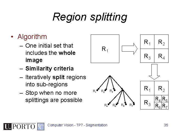
Region splitting • Algorithm – One initial set that includes the whole image – Similarity criteria – Iteratively split regions into sub-regions – Stop when no more splittings are possible R 1 R 2 R 4 Computer Vision - TP 7 - Segmentation R 3 R 5 R 6 R 7 R 1 R 2 R 3 R 4 R 5 R 6 R 7 35

Computer Vision - TP 7 - Segmentation 36 [Machine Vision; David Vernon]

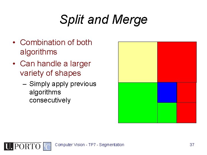
Split and Merge • Combination of both algorithms • Can handle a larger variety of shapes – Simply apply previous algorithms consecutively Computer Vision - TP 7 - Segmentation 37

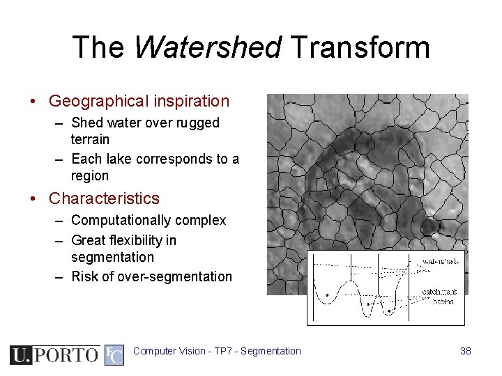
The Watershed Transform • Geographical inspiration – Shed water over rugged terrain – Each lake corresponds to a region • Characteristics – Computationally complex – Great flexibility in segmentation – Risk of over-segmentation Computer Vision - TP 7 - Segmentation 38

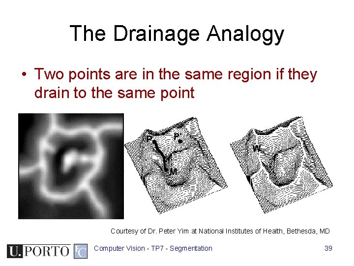
The Drainage Analogy • Two points are in the same region if they drain to the same point Courtesy of Dr. Peter Yim at National Institutes of Health, Bethesda, MD Computer Vision - TP 7 - Segmentation 39

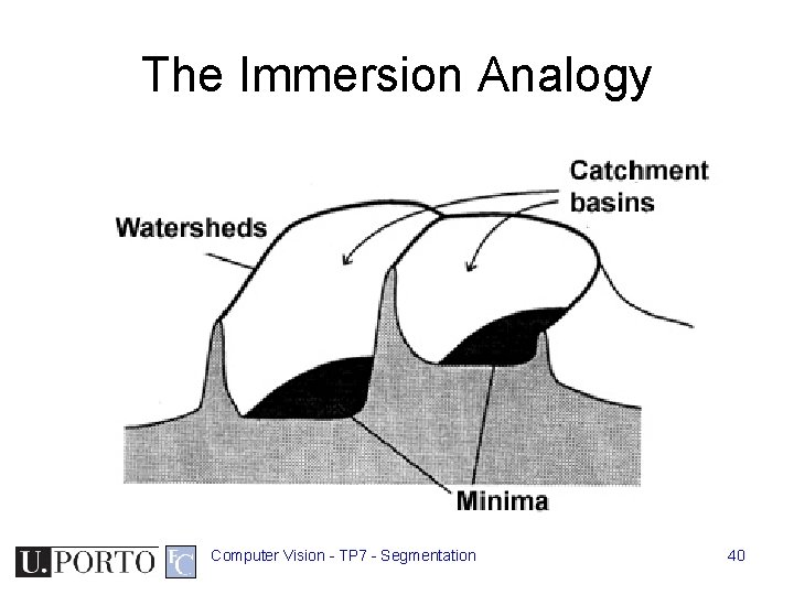
The Immersion Analogy Computer Vision - TP 7 - Segmentation 40

[Milan Sonka, Vaclav Hlavac, and Roger Boyle] Computer Vision - TP 7 - Segmentation 41

Over-Segmentation • Over-segmentation – Raw watershed segmentation produces a severely oversegmented image with hundreds or thousands of catchment basins • Post-Processing – Region merging – Edge information – Etc. Computer Vision - TP 7 - Segmentation 42

Resources • Szeliski, “Computer Vision: Algorithms and Applications”, Springer, 2011 – Chapter 5 – “Segmentation” Computer Vision - TP 7 - Segmentation 43