Computer Vision TP 6 Spatial Filters Miguel Tavares

Computer Vision – TP 6 Spatial Filters Miguel Tavares Coimbra

Outline • • Spatial filters Frequency domain filtering Edge detection Morphological filters Computer Vision - TP 6 - Spatial Filters 2

Topic: Spatial filters • • Spatial filters Frequency domain filtering Edge detection Morphological filters Computer Vision - TP 6 - Spatial Filters 3

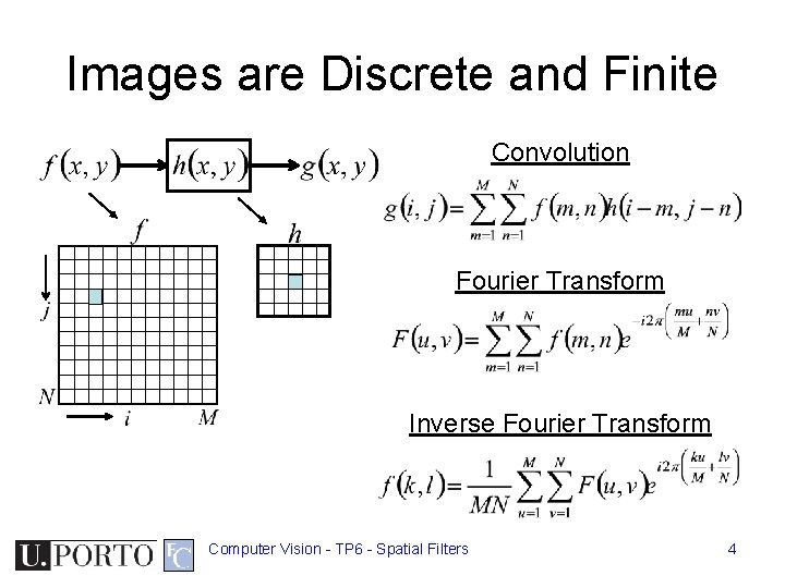
Images are Discrete and Finite Convolution Fourier Transform Inverse Fourier Transform Computer Vision - TP 6 - Spatial Filters 4

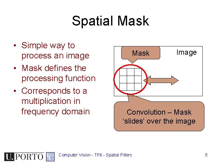
Spatial Mask • Simple way to process an image • Mask defines the processing function • Corresponds to a multiplication in frequency domain Mask Image Convolution – Mask ‘slides’ over the image Computer Vision - TP 6 - Spatial Filters 5

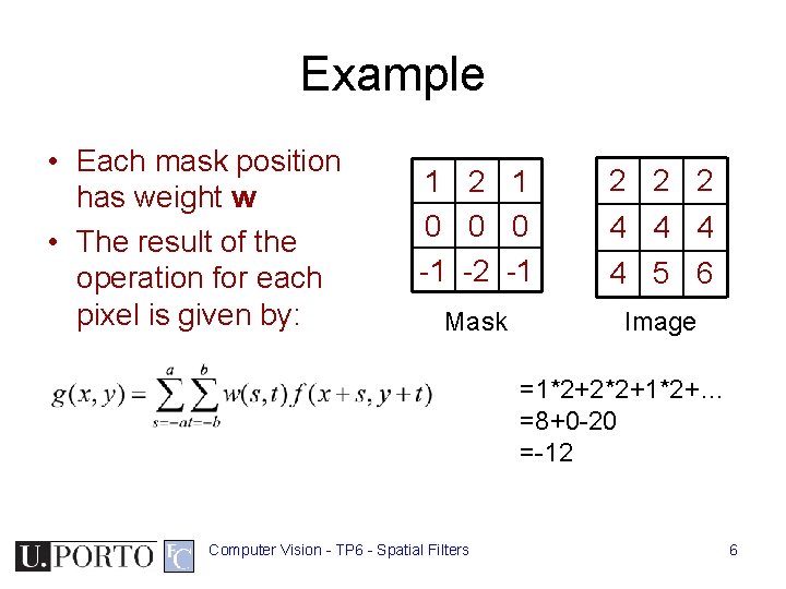
Example • Each mask position has weight w • The result of the operation for each pixel is given by: 1 2 1 0 0 0 -1 -2 -1 2 2 2 Mask Image 4 4 5 6 =1*2+2*2+1*2+… =8+0 -20 =-12 Computer Vision - TP 6 - Spatial Filters 6

Definitions • Spatial filters – Use a mask (kernel) over an image region – Work directly with pixels – As opposed to: Frequency filters • Advantages – Simplementation: convolution with the kernel function – Different masks offer a large variety of functionalities Computer Vision - TP 6 - Spatial Filters 7

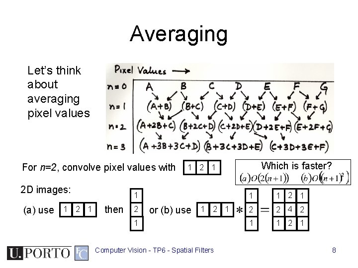
Averaging Let’s think about averaging pixel values For n=2, convolve pixel values with 2 D images: (a) use 1 2 1 1 then 2 Which is faster? 1 2 1 or (b) use 1 2 1 1 Computer Vision - TP 6 - Spatial Filters 1 1 2 2 4 2 1 1 2 1 8

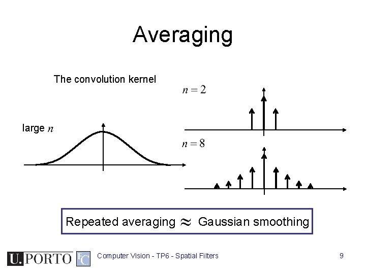
Averaging The convolution kernel large Repeated averaging Gaussian smoothing Computer Vision - TP 6 - Spatial Filters 9

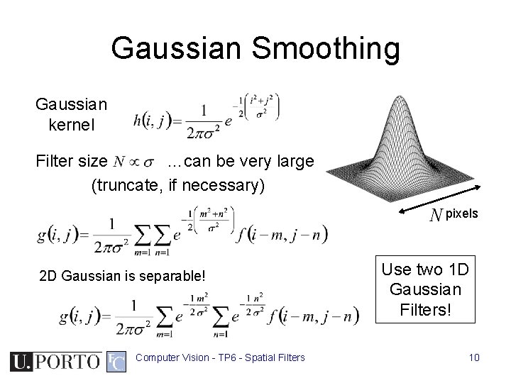
Gaussian Smoothing Gaussian kernel Filter size …can be very large (truncate, if necessary) pixels 2 D Gaussian is separable! Computer Vision - TP 6 - Spatial Filters Use two 1 D Gaussian Filters! 10

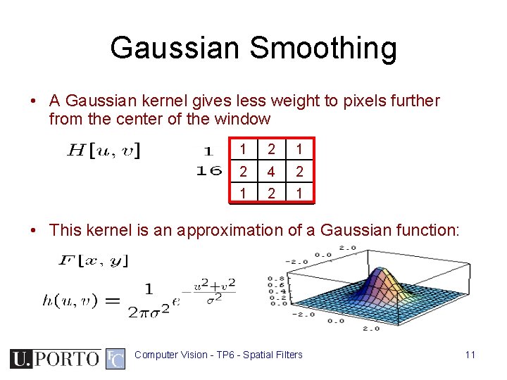
Gaussian Smoothing • A Gaussian kernel gives less weight to pixels further from the center of the window 1 2 4 2 1 • This kernel is an approximation of a Gaussian function: Computer Vision - TP 6 - Spatial Filters 11

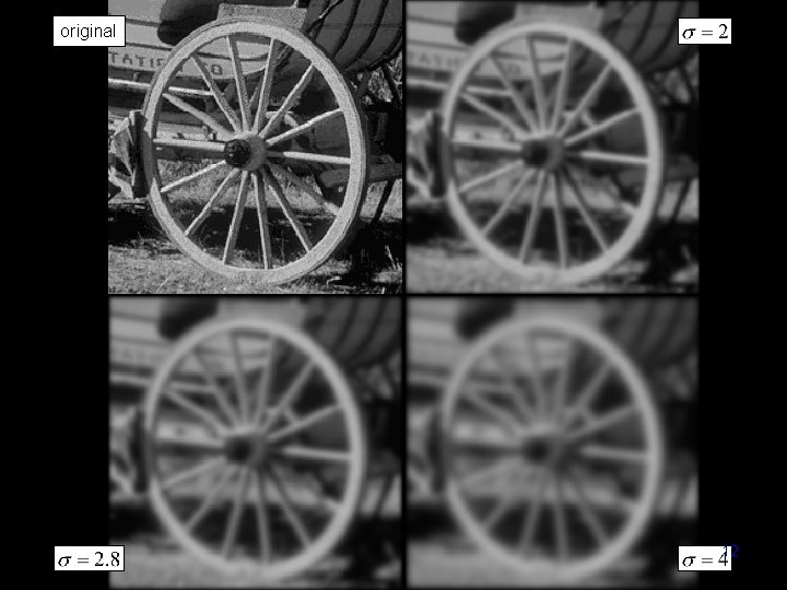
original Computer Vision - TP 6 - Spatial Filters 12

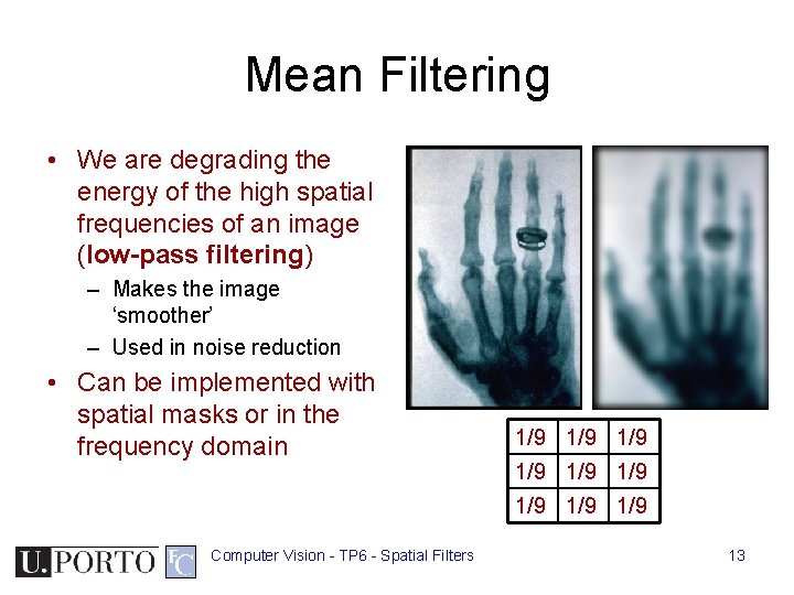
Mean Filtering • We are degrading the energy of the high spatial frequencies of an image (low-pass filtering) – Makes the image ‘smoother’ – Used in noise reduction • Can be implemented with spatial masks or in the frequency domain 1/9 1/9 1/9 Computer Vision - TP 6 - Spatial Filters 13

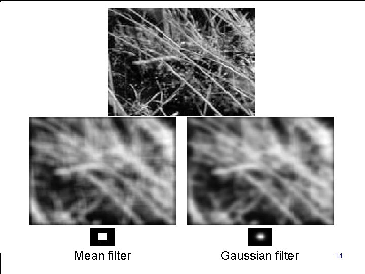
Computer Mean filter. Vision - TP 6 - Spatial Filters Gaussian filter 14

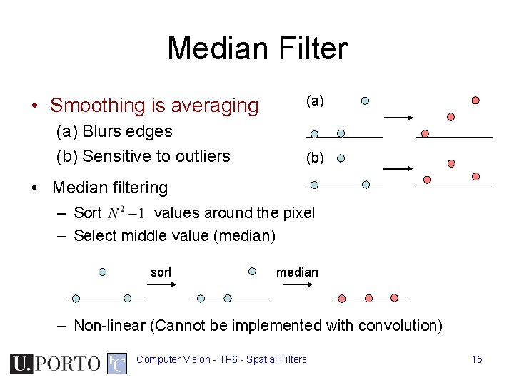
Median Filter • Smoothing is averaging (a) Blurs edges (b) Sensitive to outliers (a) (b) • Median filtering – Sort values around the pixel – Select middle value (median) sort median – Non-linear (Cannot be implemented with convolution) Computer Vision - TP 6 - Spatial Filters 15

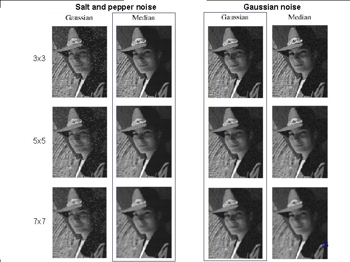
Salt and pepper noise Gaussian noise 3 x 3 5 x 5 7 x 7 Computer Vision - TP 6 - Spatial Filters 16

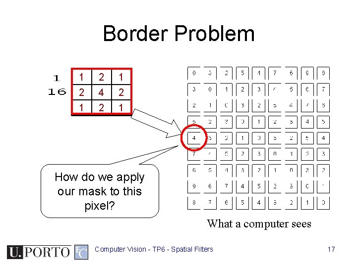
Border Problem 1 2 4 2 1 How do we apply our mask to this pixel? What a computer sees Computer Vision - TP 6 - Spatial Filters 17

Border Problem • Ignore – Output image will be smaller than original • Pad with constant values – Can introduce substantial 1 st order derivative values • Pad with reflection – Can introduce substantial 2 nd order derivative values Computer Vision - TP 6 - Spatial Filters 18

Topic: Frequency domain filtering • • Spatial filters Frequency domain filtering Edge detection Morphological filters Computer Vision - TP 6 - Spatial Filters 19

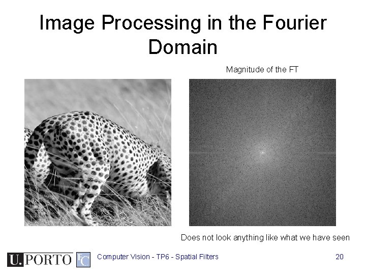
Image Processing in the Fourier Domain Magnitude of the FT Does not look anything like what we have seen Computer Vision - TP 6 - Spatial Filters 20

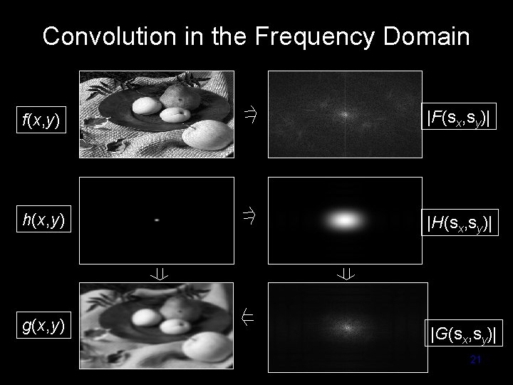
Convolution in the Frequency Domain f(x, y) |F(sx, sy)| h(x, y) |H(sx, sy)| g(x, y) |G(sx, sy)| Computer Vision - TP 6 - Spatial Filters 21

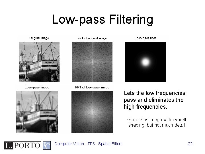
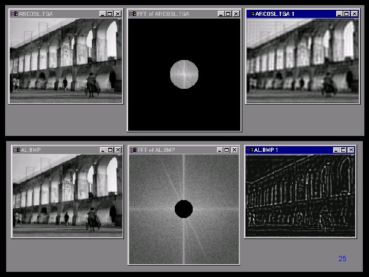
Low-pass Filtering Lets the low frequencies pass and eliminates the high frequencies. Generates image with overall shading, but not much detail Computer Vision - TP 6 - Spatial Filters 22

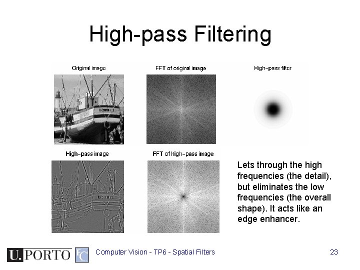
High-pass Filtering Lets through the high frequencies (the detail), but eliminates the low frequencies (the overall shape). It acts like an edge enhancer. Computer Vision - TP 6 - Spatial Filters 23

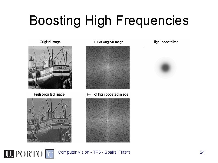
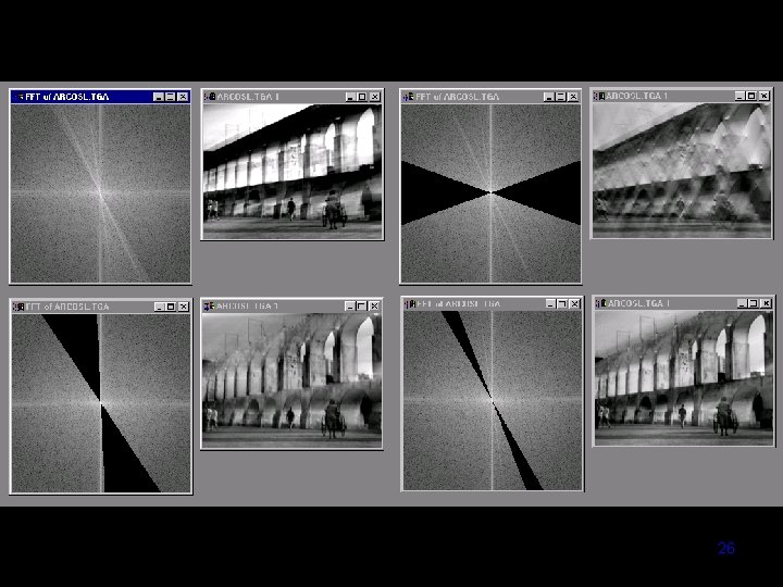
Boosting High Frequencies Computer Vision - TP 6 - Spatial Filters 24

Computer Vision - TP 6 - Spatial Filters 25

Computer Vision - TP 6 - Spatial Filters 26

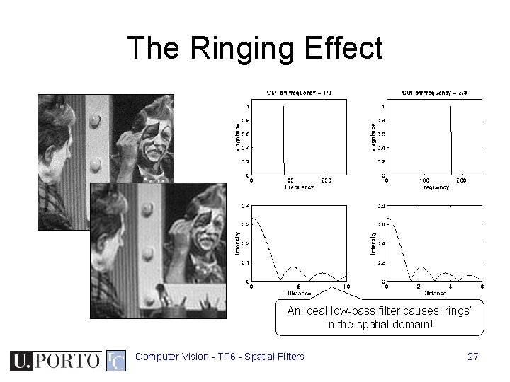
The Ringing Effect An ideal low-pass filter causes ‘rings’ in the spatial domain! Computer Vision - TP 6 - Spatial Filters 27

Topic: Edge detection • • Spatial filters Frequency domain filtering Edge detection Morphological filters Computer Vision - TP 6 - Spatial Filters 28

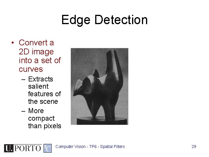
Edge Detection • Convert a 2 D image into a set of curves – Extracts salient features of the scene – More compact than pixels Computer Vision - TP 6 - Spatial Filters 29

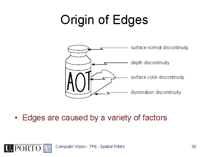
Origin of Edges surface normal discontinuity depth discontinuity surface color discontinuity illumination discontinuity • Edges are caused by a variety of factors Computer Vision - TP 6 - Spatial Filters 30

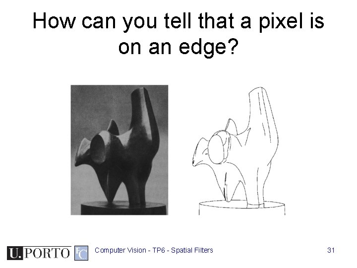
How can you tell that a pixel is on an edge? Computer Vision - TP 6 - Spatial Filters 31

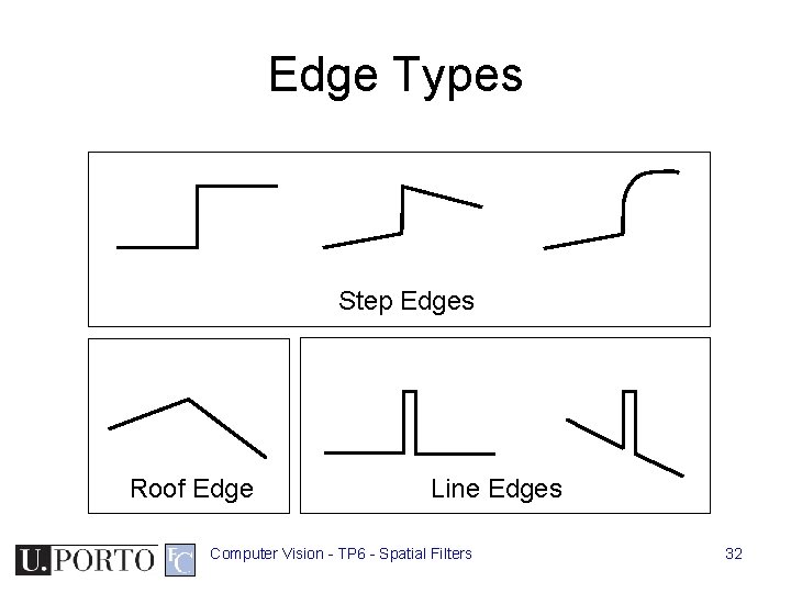
Edge Types Step Edges Roof Edge Line Edges Computer Vision - TP 6 - Spatial Filters 32

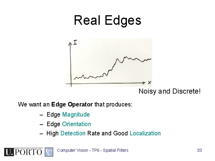
Real Edges Noisy and Discrete! We want an Edge Operator that produces: – Edge Magnitude – Edge Orientation – High Detection Rate and Good Localization Computer Vision - TP 6 - Spatial Filters 33

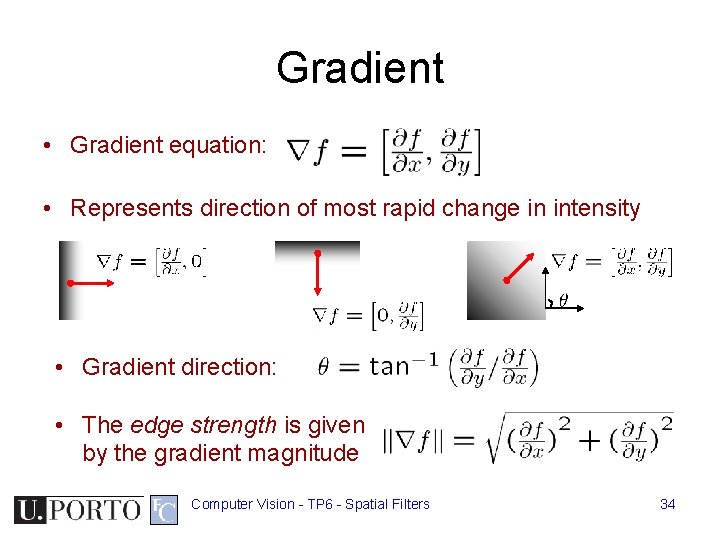
Gradient • Gradient equation: • Represents direction of most rapid change in intensity • Gradient direction: • The edge strength is given by the gradient magnitude Computer Vision - TP 6 - Spatial Filters 34

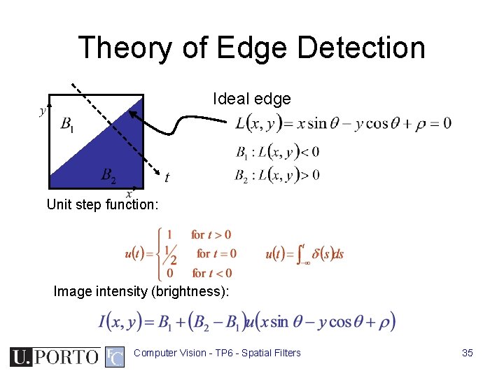
Theory of Edge Detection Ideal edge Unit step function: Image intensity (brightness): Computer Vision - TP 6 - Spatial Filters 35

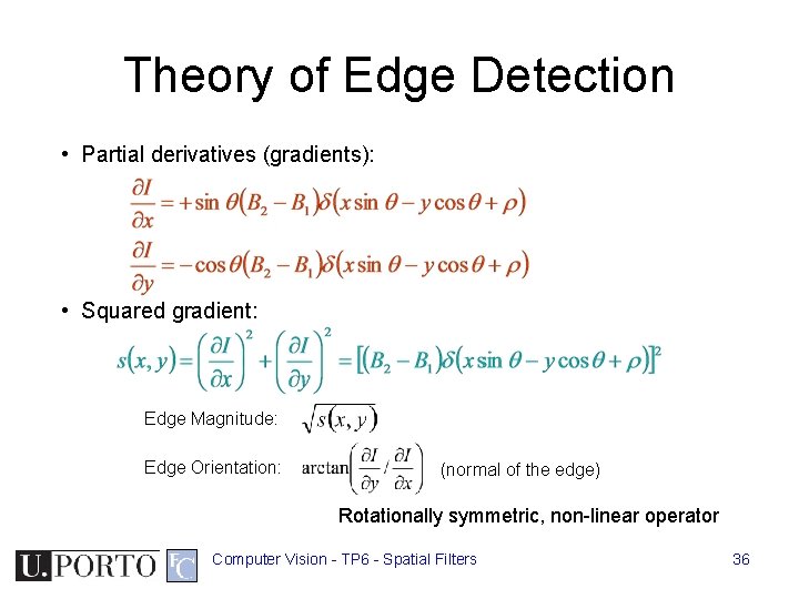
Theory of Edge Detection • Partial derivatives (gradients): • Squared gradient: Edge Magnitude: Edge Orientation: (normal of the edge) Rotationally symmetric, non-linear operator Computer Vision - TP 6 - Spatial Filters 36

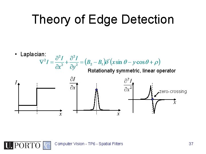
Theory of Edge Detection • Laplacian: Rotationally symmetric, linear operator zero-crossing Computer Vision - TP 6 - Spatial Filters 37

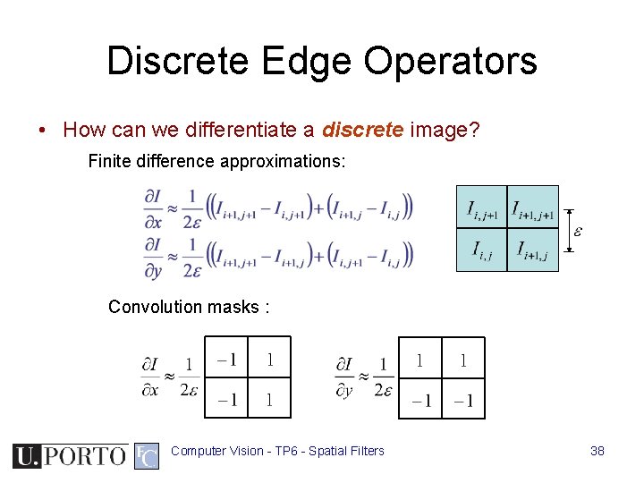
Discrete Edge Operators • How can we differentiate a discrete image? Finite difference approximations: Convolution masks : Computer Vision - TP 6 - Spatial Filters 38

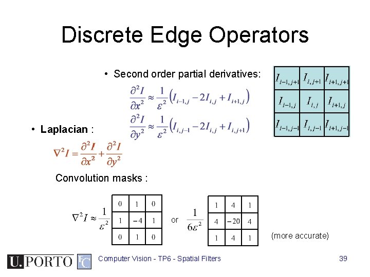
Discrete Edge Operators • Second order partial derivatives: • Laplacian : Convolution masks : or (more accurate) Computer Vision - TP 6 - Spatial Filters 39

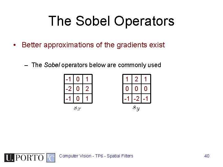
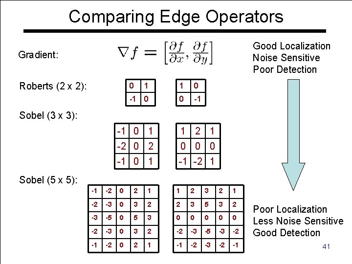
The Sobel Operators • Better approximations of the gradients exist – The Sobel operators below are commonly used -1 0 1 1 2 1 -2 0 0 0 -1 0 1 -1 -2 -1 Computer Vision - TP 6 - Spatial Filters 40

Comparing Edge Operators Good Localization Noise Sensitive Poor Detection Gradient: Roberts (2 x 2): 0 1 1 0 -1 0 0 -1 Sobel (3 x 3): -1 0 1 1 2 1 -2 0 0 0 -1 0 1 -1 -2 1 Sobel (5 x 5): -1 -2 0 2 1 1 2 3 2 1 -2 -3 0 3 2 2 3 5 3 2 -3 -5 0 5 3 0 0 0 -2 -3 0 3 2 -2 -3 -5 -3 -2 -1 -2 0 Vision 2 -1 TP 6 - Spatial -1 -2 -3 Computer Filters -2 -1 Poor Localization Less Noise Sensitive Good Detection 41

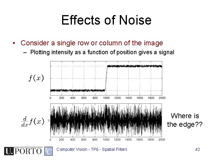
Effects of Noise • Consider a single row or column of the image – Plotting intensity as a function of position gives a signal Where is the edge? ? Computer Vision - TP 6 - Spatial Filters 42

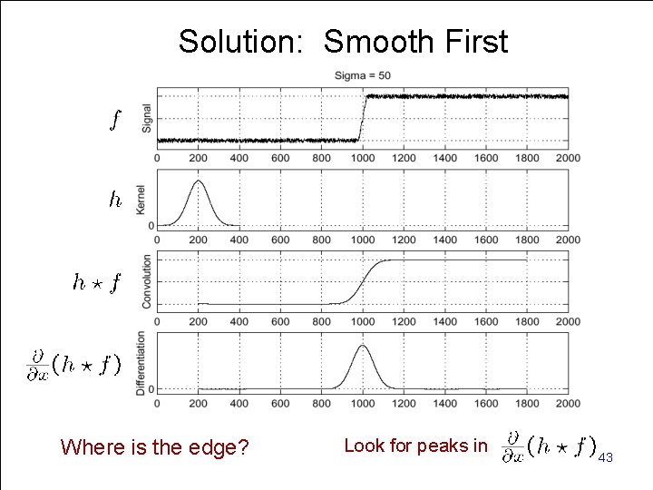
Solution: Smooth First Look for peaks in Where is the. Computer edge? Vision - TP 6 - Spatial Filters 43

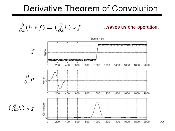
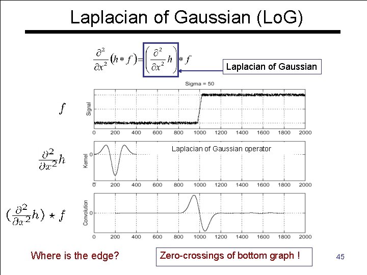
Derivative Theorem of Convolution …saves us one operation. Computer Vision - TP 6 - Spatial Filters 44

Laplacian of Gaussian (Lo. G) Laplacian of Gaussian operator Zero-crossings Computer Vision - TP 6 - Spatial Filters of bottom graph ! Where is the edge? 45

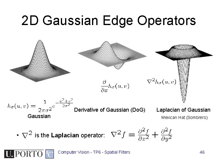
2 D Gaussian Edge Operators Derivative of Gaussian (Do. G) Gaussian • Laplacian of Gaussian Mexican Hat (Sombrero) is the Laplacian operator: Computer Vision - TP 6 - Spatial Filters 46

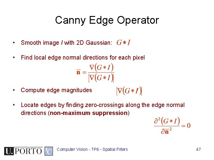
Canny Edge Operator • Smooth image I with 2 D Gaussian: • Find local edge normal directions for each pixel • Compute edge magnitudes • Locate edges by finding zero-crossings along the edge normal directions (non-maximum suppression) Computer Vision - TP 6 - Spatial Filters 47

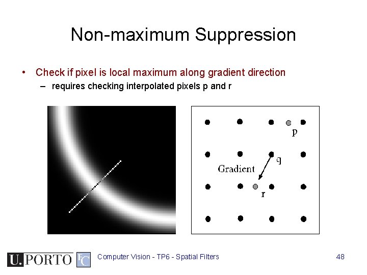
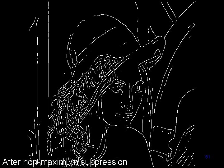
Non-maximum Suppression • Check if pixel is local maximum along gradient direction – requires checking interpolated pixels p and r Computer Vision - TP 6 - Spatial Filters 48

original image Computer Vision - TP 6 - Spatial Filters 49

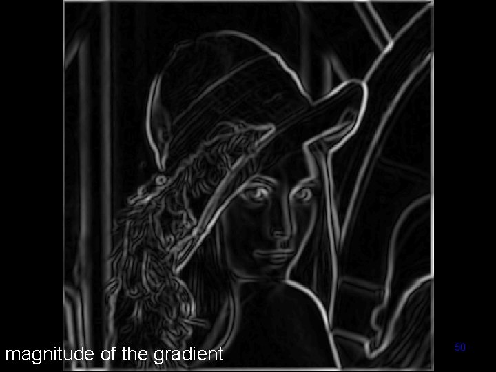
Computer Vision - TP 6 - Spatial Filters magnitude of the gradient 50

Computer Vision - TP 6 - Spatial Filters After non-maximum suppression 51

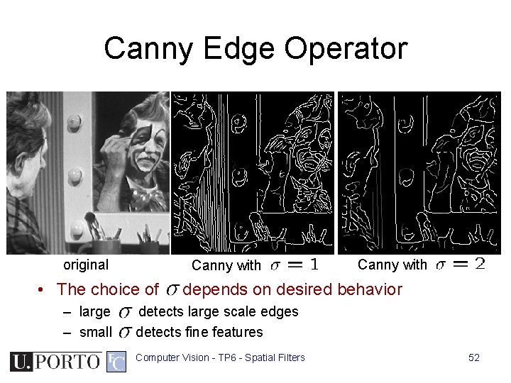
Canny Edge Operator original Canny with • The choice of – large – small Canny with depends on desired behavior detects large scale edges detects fine features Computer Vision - TP 6 - Spatial Filters 52

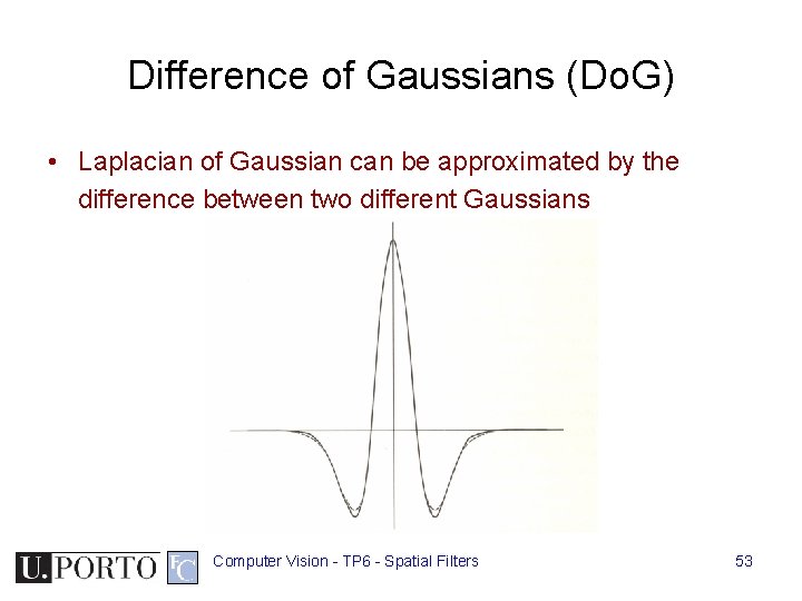
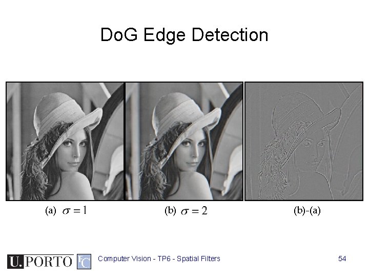
Difference of Gaussians (Do. G) • Laplacian of Gaussian can be approximated by the difference between two different Gaussians Computer Vision - TP 6 - Spatial Filters 53

Do. G Edge Detection (a) (b) Computer Vision - TP 6 - Spatial Filters (b)-(a) 54

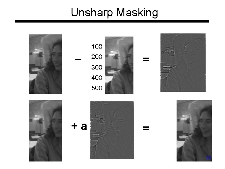
Unsharp Masking – = +a = Computer Vision - TP 6 - Spatial Filters 55

Topic: Morphological Filters • • Spatial filters Frequency domain filtering Edge detection Morphological filters Computer Vision - TP 6 - Spatial Filters 56

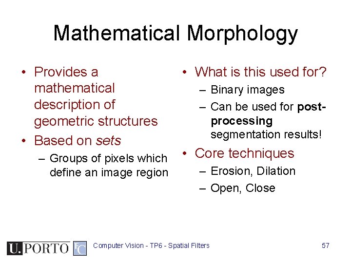
Mathematical Morphology • Provides a mathematical description of geometric structures • Based on sets – Groups of pixels which define an image region • What is this used for? – Binary images – Can be used for postprocessing segmentation results! • Core techniques – Erosion, Dilation – Open, Close Computer Vision - TP 6 - Spatial Filters 57

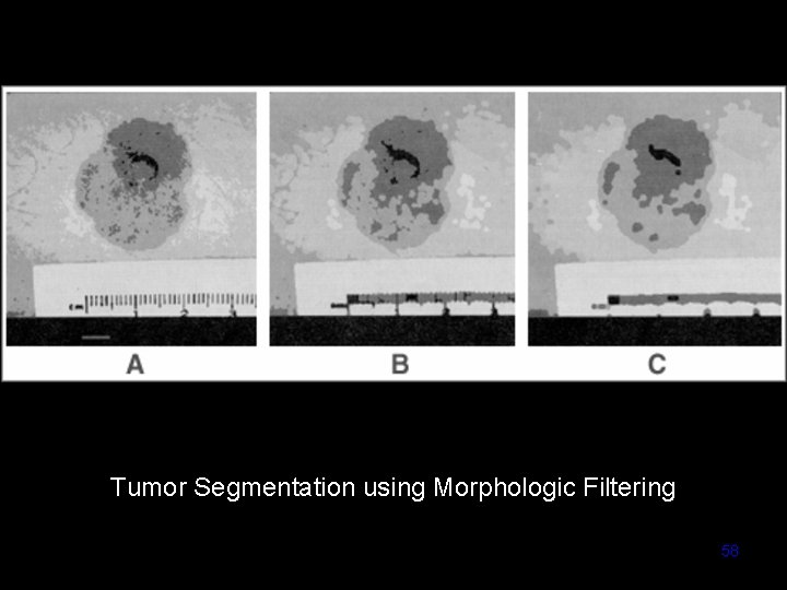
Tumor Segmentation using Morphologic Filtering Computer Vision - TP 6 - Spatial Filters 58

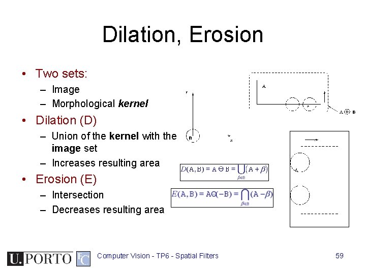
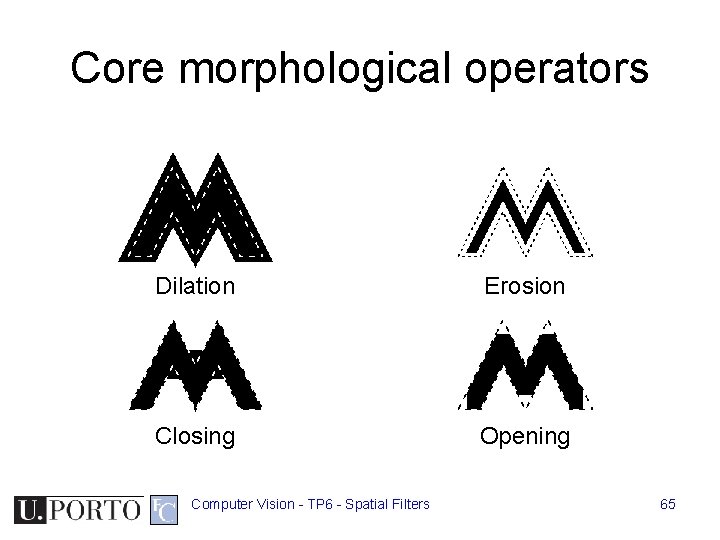
Dilation, Erosion • Two sets: – Image – Morphological kernel • Dilation (D) – Union of the kernel with the image set – Increases resulting area • Erosion (E) – Intersection – Decreases resulting area Computer Vision - TP 6 - Spatial Filters 59

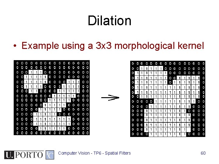
Dilation • Example using a 3 x 3 morphological kernel Computer Vision - TP 6 - Spatial Filters 60

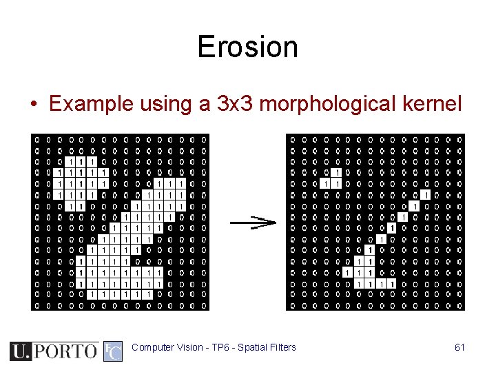
Erosion • Example using a 3 x 3 morphological kernel Computer Vision - TP 6 - Spatial Filters 61

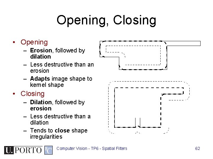
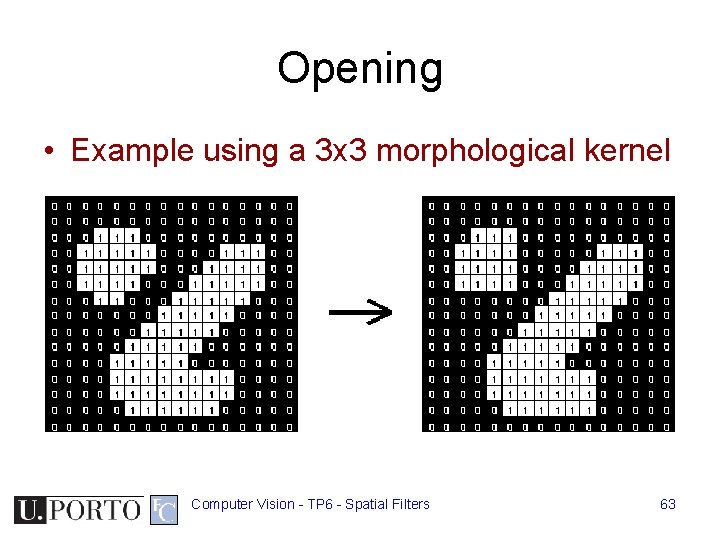
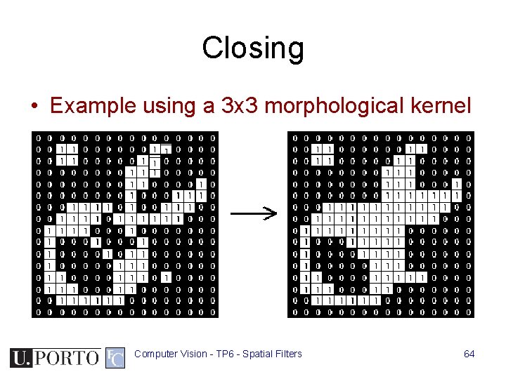
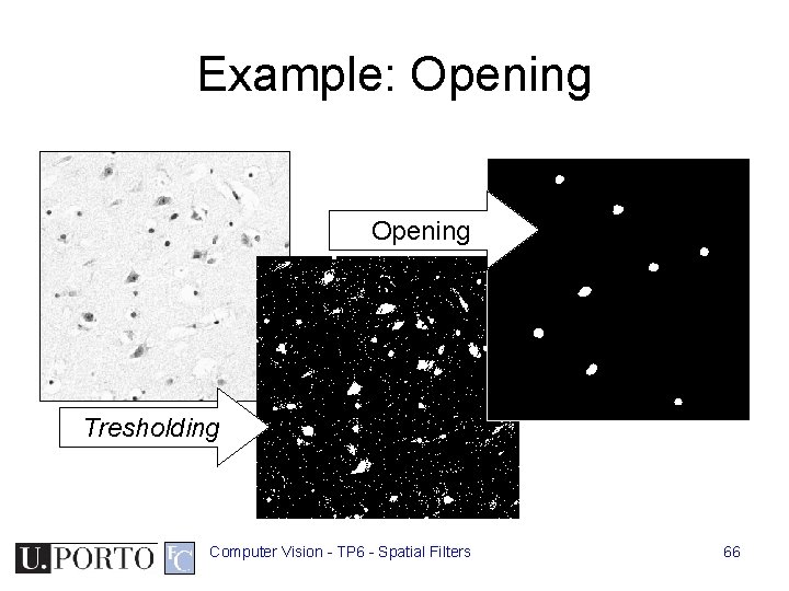
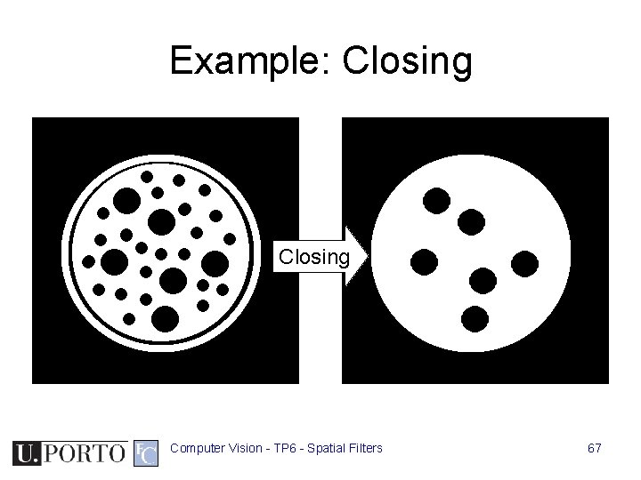
Opening, Closing • Opening – Erosion, followed by dilation – Less destructive than an erosion – Adapts image shape to kernel shape • Closing – Dilation, followed by erosion – Less destructive than a dilation – Tends to close shape irregularities Computer Vision - TP 6 - Spatial Filters 62

Opening • Example using a 3 x 3 morphological kernel Computer Vision - TP 6 - Spatial Filters 63

Closing • Example using a 3 x 3 morphological kernel Computer Vision - TP 6 - Spatial Filters 64

Core morphological operators Dilation Erosion Closing Opening Computer Vision - TP 6 - Spatial Filters 65

Example: Opening Tresholding Computer Vision - TP 6 - Spatial Filters 66

Example: Closing Computer Vision - TP 6 - Spatial Filters 67

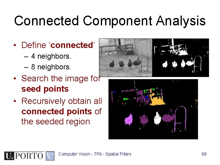
Connected Component Analysis • Define ‘connected’ – 4 neighbors. – 8 neighbors. • Search the image for seed points • Recursively obtain all connected points of the seeded region Computer Vision - TP 6 - Spatial Filters 68

Resources • Szeliski, “Computer Vision: Algorithms and Applications”, Springer, 2011 – Chapter 3 – “Image Processing” – Chapter 4 – “Feature Detection and Matching” Computer Vision - TP 6 - Spatial Filters 69